If you know my #WarTraces post, you’ll see that I use satellite imagery from the European Space Agency. Today I’ll show how to download and manipulate these images from mission Sentinel 2, as well as Landsat, being very similar to do.
I’ll do it in QGIS, so you need to download this software with the GRASS GIS module included.
Content
Sign up in platforms.
You need to create an account to access both data sources, just filling a form and confirming via email.
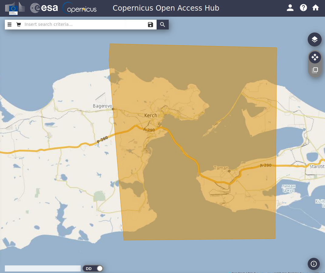
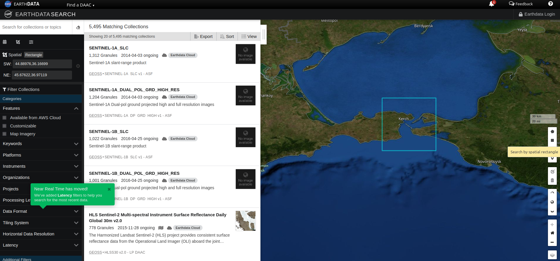
Now, draw a delimiting polygon of the area of interest. Every corner is set with right click, and the polygon is closed with double right click.
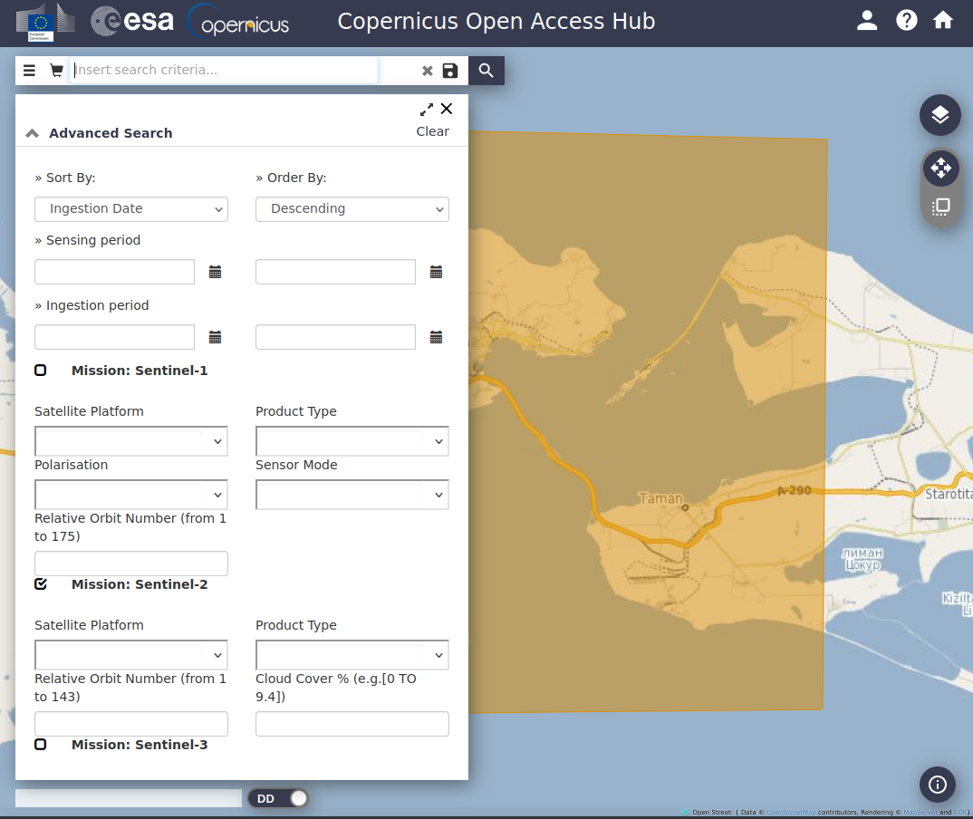
Next, click the filter icon in the search bar and tick the box for mission Sentinel-2 (you can also set dates, but it will be sorted from recent to old by default).
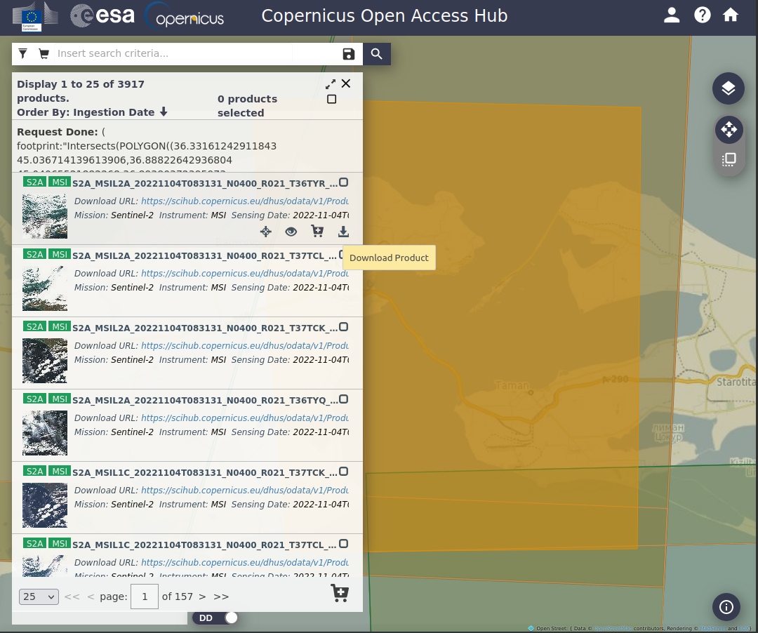
Finally, all available products will appear, so you can preview or download in a compressed .zip file.
Define an area of interest using the geometry tools in the lateral bar.
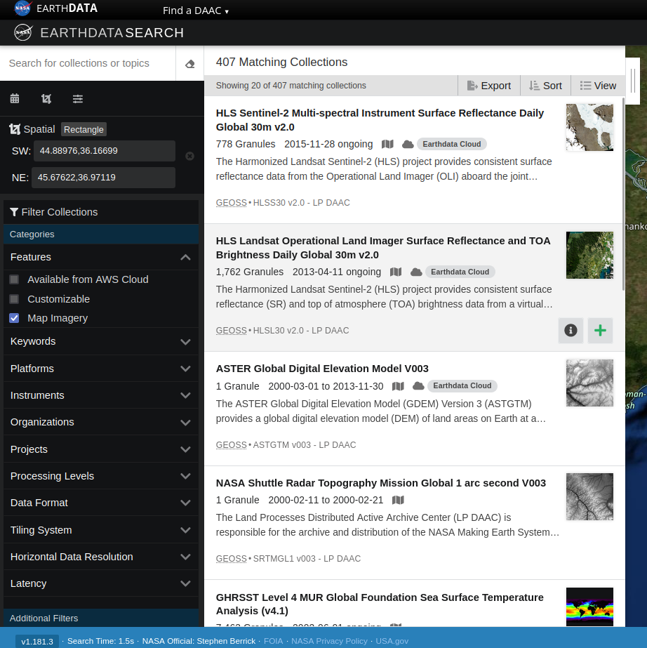
Filter the products, for example selecting "Imagery". Then select the HLS Landsat dataset in the catalogue.
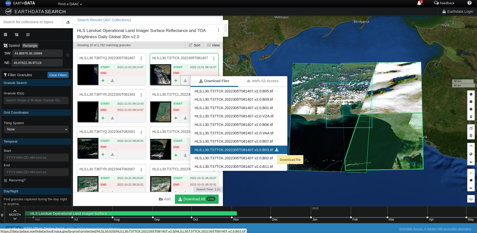
In this case, we need to download each band separately, which we'll see next.
TCI image (true colour)
Simplifying (a lot), satellites capture images in different wave longitude ranges, called bands.
Also, digital images or pictures that we use to represent reality seen by the naked eye use to be defined in three layers: one for color Red, another for color Green, and another one for Blue, defining in each of these layers one value for every pixel with the amount of this color. The combination of all pixels is what simulates an image similar to reality.
TIP! Do the test and zoom in a lot in any picture and see the mosaic of pixels that make it up.
Lets use the bands captured by satellites in the visible wave range to generate an image as if we saw it from space.
Sentinel 2
In the case of Sentinel 2, we can show a true color image directly downloading the product L1C and using the layer _TCI.jp2 located in /GRANULE/DATASET_CODE_NAME/IMG_DATA/
The TCI image will show like this:
Deir ez Zor, Syria, 22/10/2017. TCI. Source: Copernicus Sentinel 2.
For Landsat, we need to combine the different bands captured individually by the satellite in the visible wave range. These are:
RED
B04
GREEN
B03
BLUE
B02
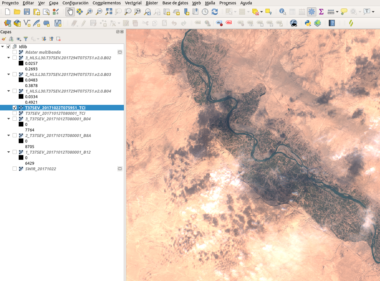
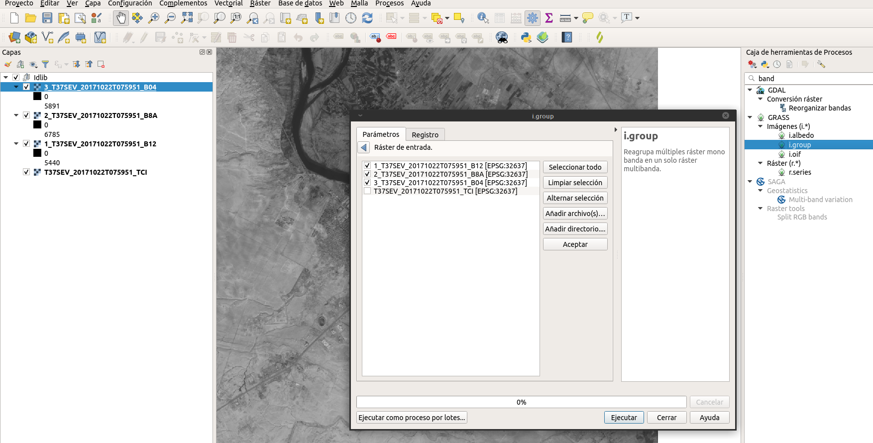
Now in QGIS, we'll use function i.group from GRASS module which combines the selected layers in a multiband Red, Green, Blue layer.
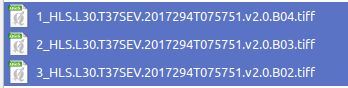
To make it easier, I rename the layers like this, to make sure the script reads them properly:
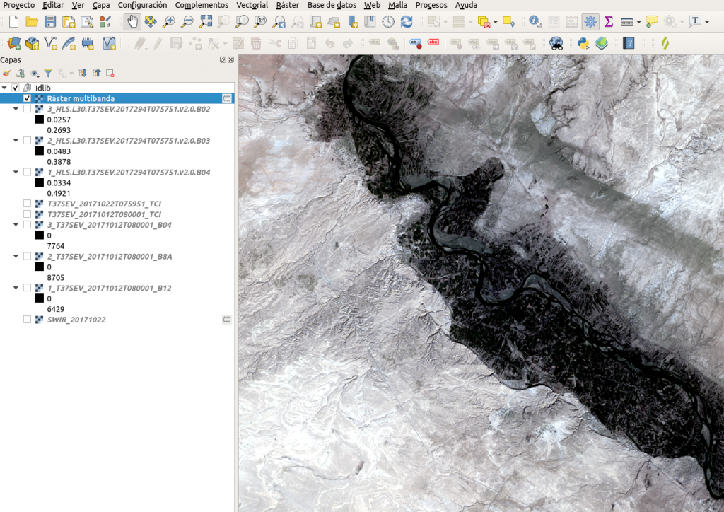
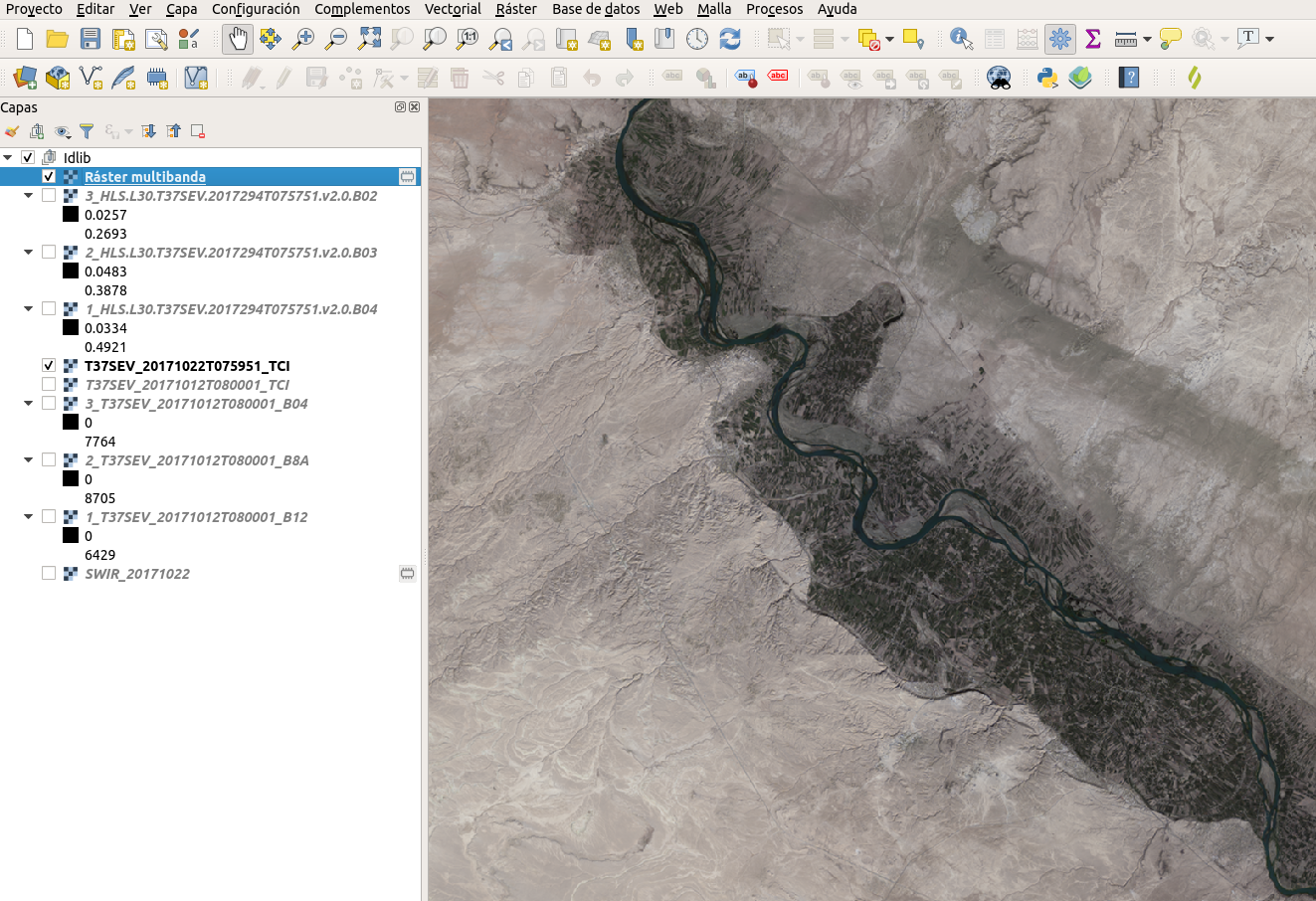
Looking like this:
In this case it's nothing similar to the previous image or reality, so we'll adjust the properties to extract more color from the data:
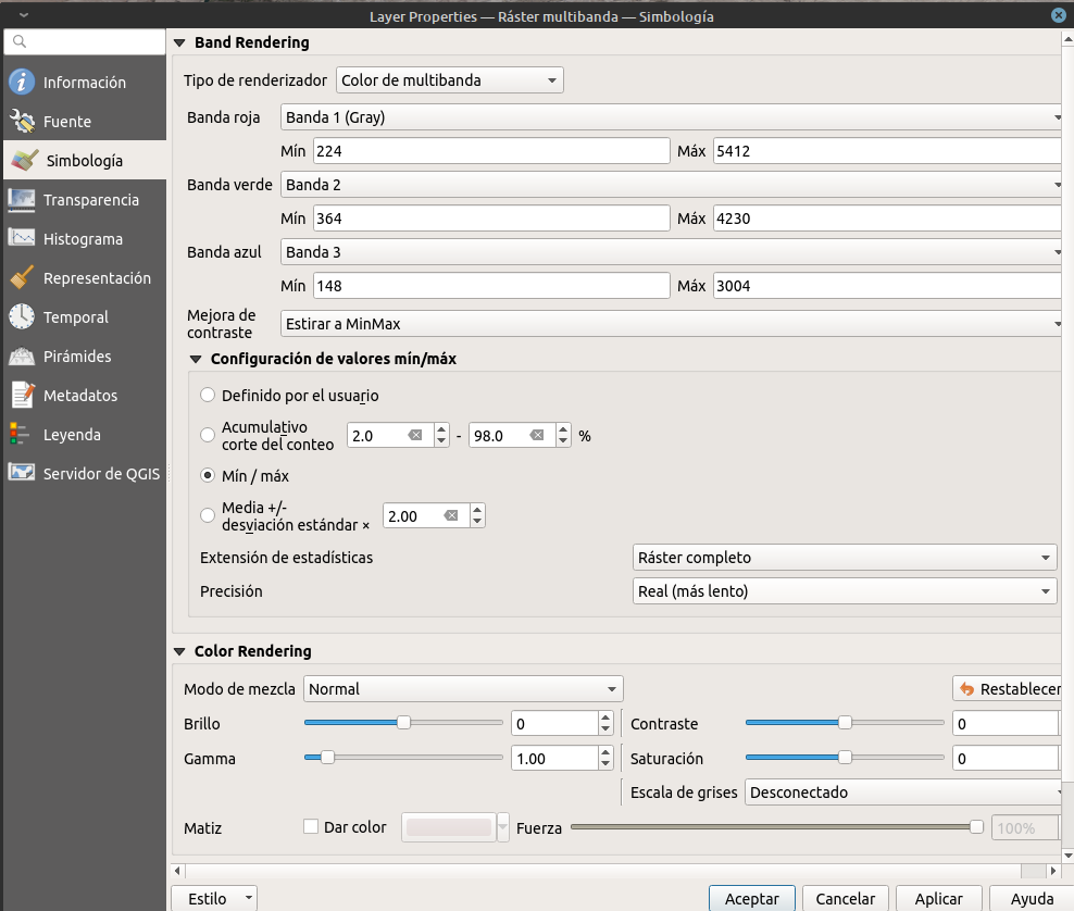
First, let's make sure we use all the data reading real max/min values rather than estimated.
The image already looks better, but missing some brightness and color.
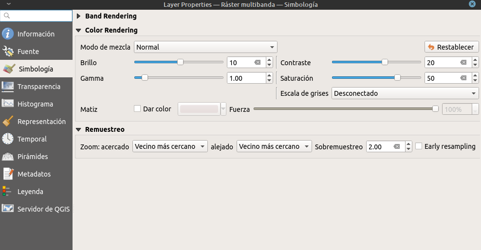
So let's adjust Color Rendering parameters:
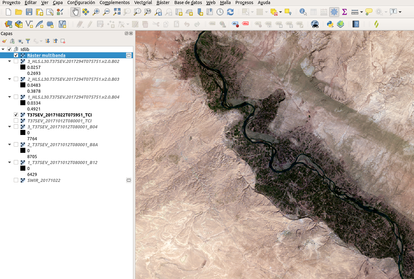
And it now looks more realistic:
Deir ez Zor, Siria, 21/10/2017. TCI. Source: Landsat.
SWIR (short wave infra-red)
Using bands in infra-red wave length, we can see further more than with the naked eye, or even across certain objects like some clouds or smoke.
During summer wildfires, I saw how Copernicus used these images to trace the extent of fires, and I thought they could be used to locate bomb impacts under the smoke they produce. That's how this ended in #WarTraces.
Sentinel 2
Using the process above, now we combine the following bands:
RED
B12
GREEN
B8A
BLUE
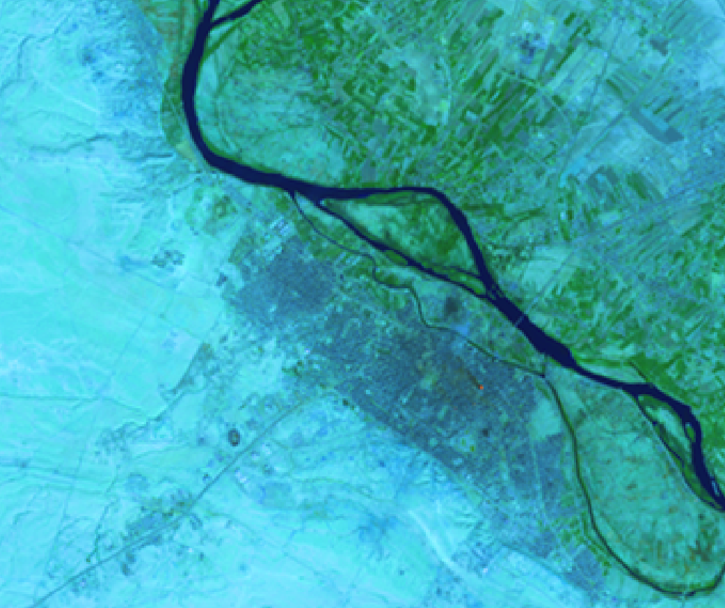
B04
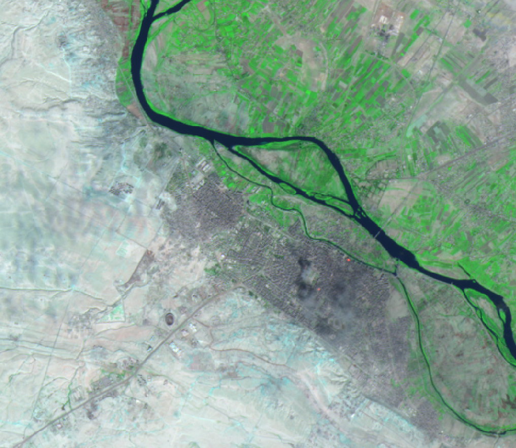
Deir ez Zor, Syria, 22/10/2017. SWIR. Source: Copernicus Sentinel 2.
Landsat
Make a new combination of these bands:
RED
B07
GREEN
B06
BLUE
B04
Deir ez Zor, Syria, 21/10/2017. SWIR. Source: Landsat.
Conclusion
As a final note, it's important to highlight the pixel size, as it will affect image detail (resolution):
Sentinel 2: 10 meters.
Landsat: 30 meters.
On the other hand, Landsat provides images since 2013, while Sentinel only provides data from 2015.
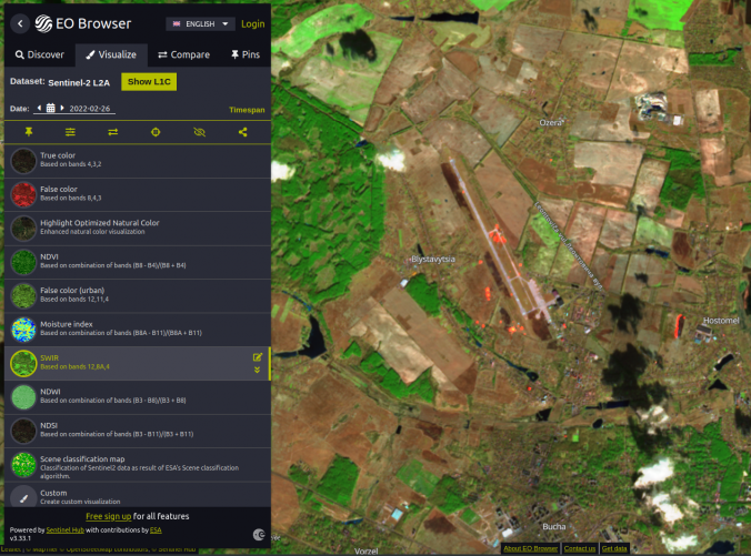
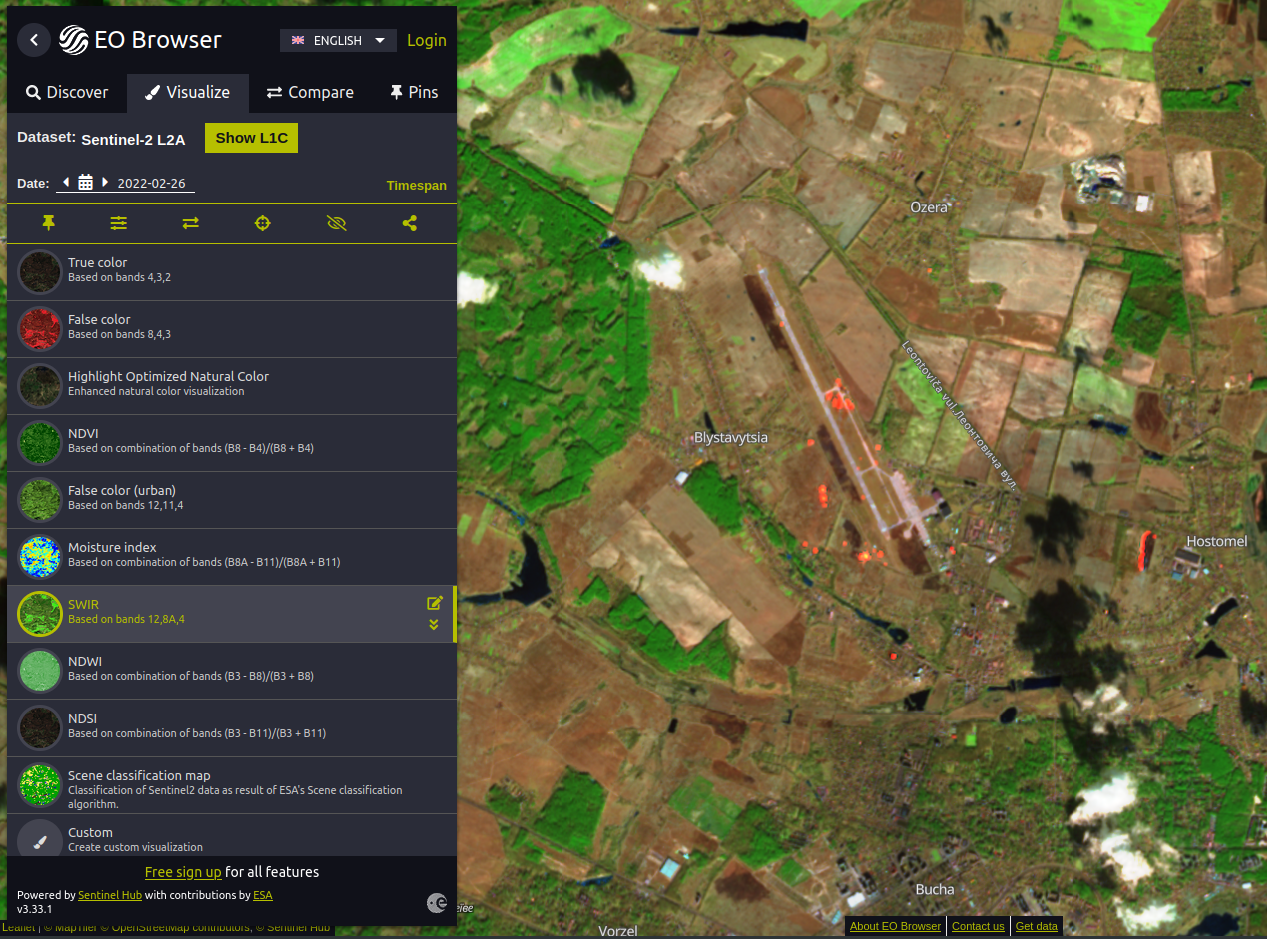
Also, you can preview all these layers and combinations in online viewers like EO Browser by Sentinel Hub.
Bombings in Antonov International Airport, Kyiv, Ukraine, 26/2/2022 using EO Browser.
If you get stuck or want to comment, let me know on 🐦 Twitter!
Blender is (to me), the top free 3D modelling software. It’s got a huge community, tones of documentation, tutorials and, overall, continuous updates and improvement.
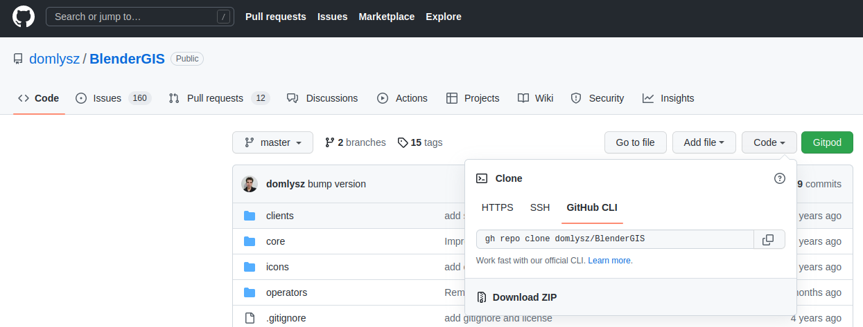
One of the most useful tools is BlenderGIS, an external plugin that lets us drop geographical data, georeferenced or not, and model with them.
Let’s see a use case with an elevation model.
Content
Installation
First thing to do is to download and install Blender from an official source (their website) or from our OS app store:
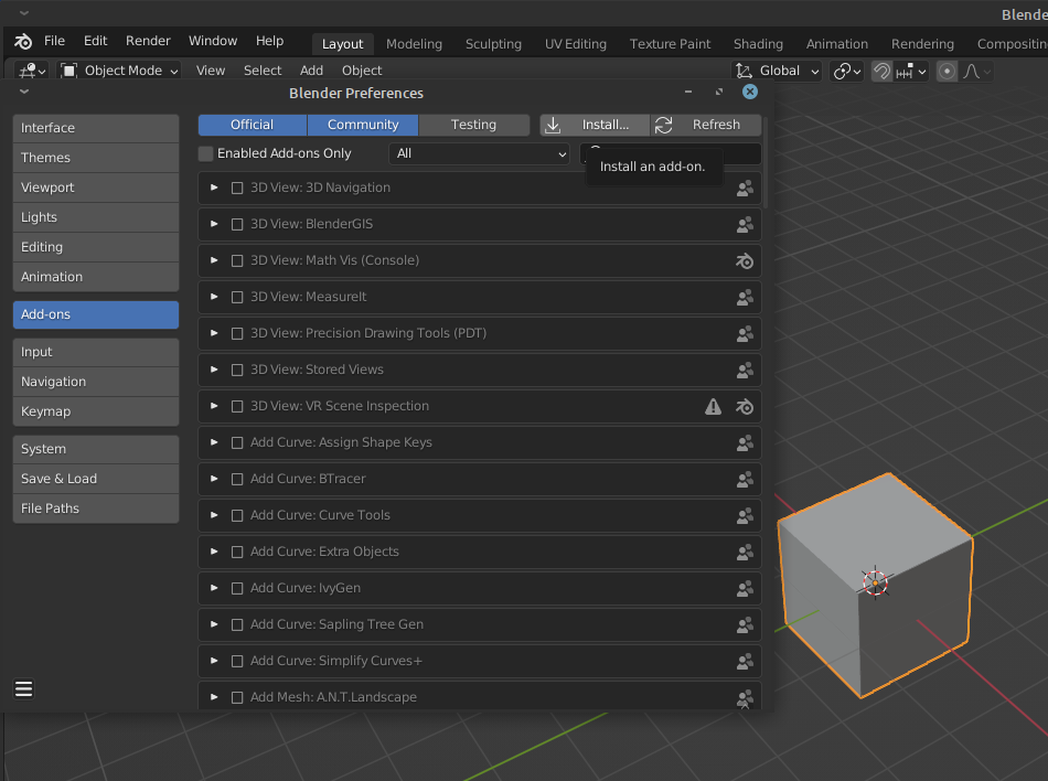
Let's now start Blender and open Add-ons settings (Edit > Preferences > Add-ons).
Press "Install..." and select the BlenderGIS .zip file.
Now you can search it and activate it.
You'll see there's a new "GIS" option in Blender's top bar.
Download geographical information
In this example I will use a Digital Terrain Model in ASCII format (.asc), as it is one of the working formats for BlenderGIS and also the standard for my download source.
If the information you download is in another format, like .tiff or .xyz, you can convert it using some software like QGIS or ArcGIS.
MDT
In my case, I will use MDT200 from spanish IGN, a terrain model with 200m cell size, as I want to show quite a large area that includes the province of Álava.
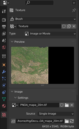
We can also use an orthophoto as a terrain texture. For this, I will be using QGIS and I will load a WMS also from IGN so I can clip the satellite image exactly to the terrain tile extent.
Load the orthophoto and the terrain layers, then export the orthophoto layer as a rendered image and set the extension from the terrain layer. I will set the cell size to 20 meters (although the imagery allows up to 20cm cell size, which would result in a huge file; the 20m image is already 140MB).
TIP! One way to optimize detail is to generate a grid of smaller size images but higher resolution.
Modelling in Blender
Now it's all ready for Blender.
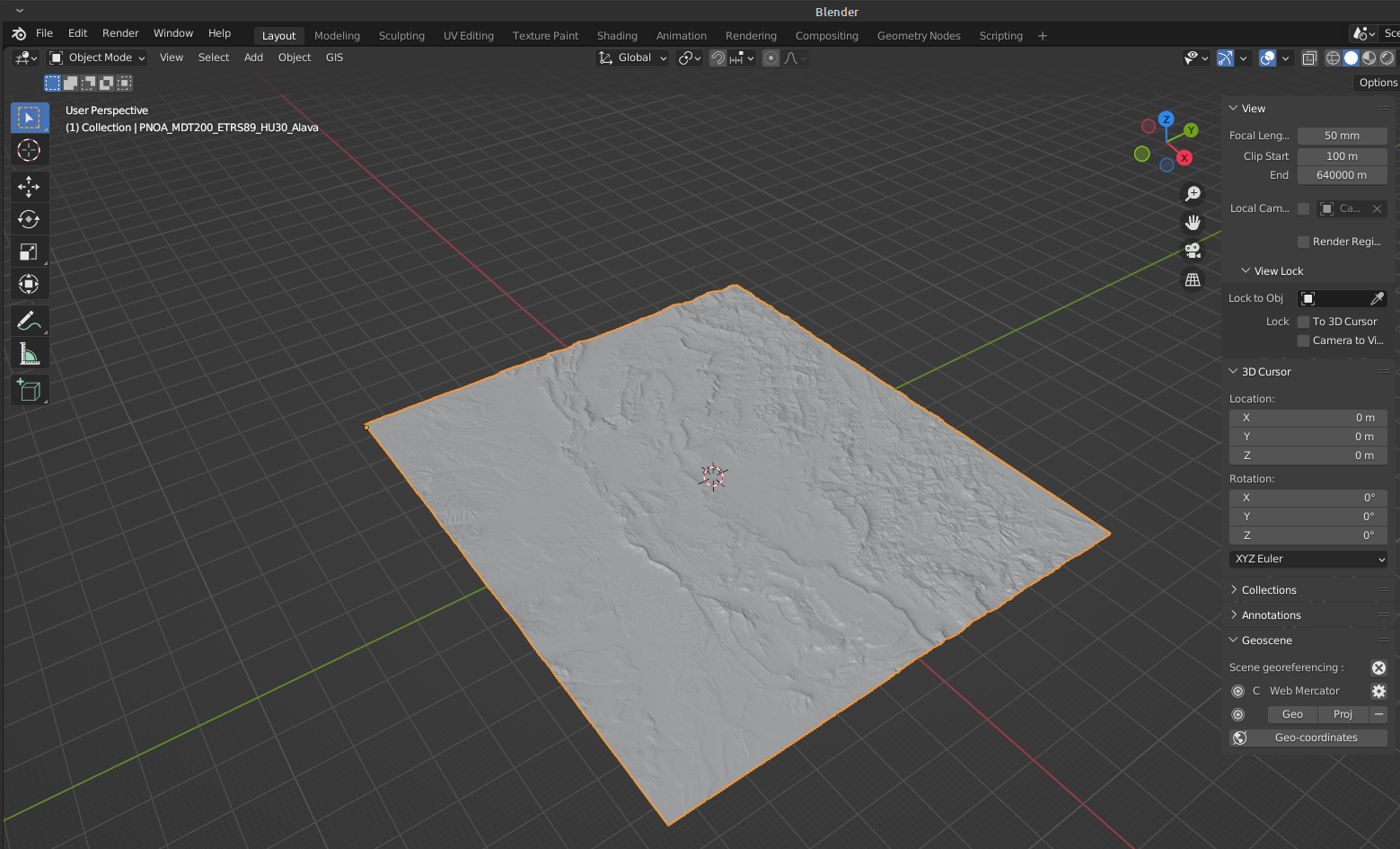
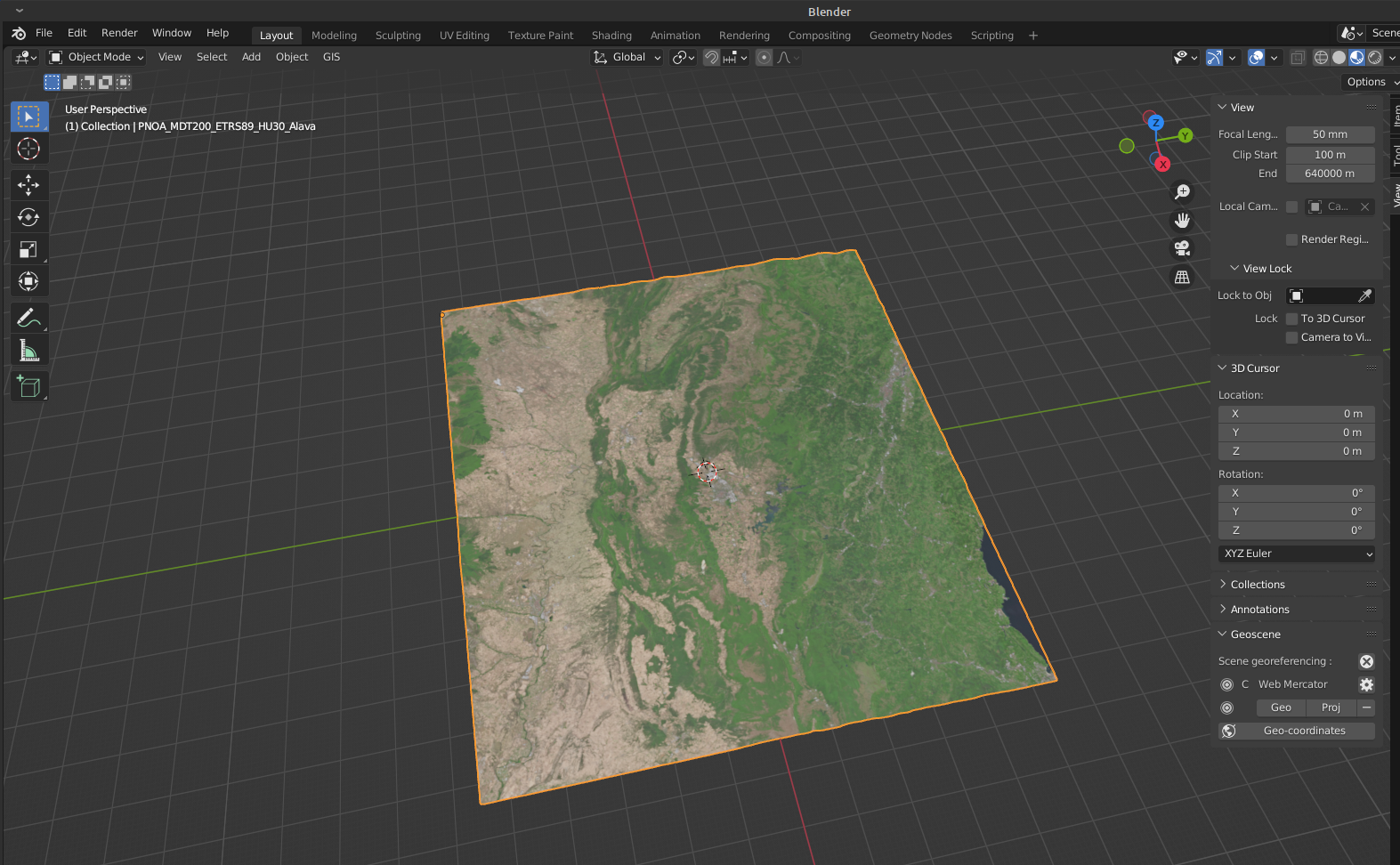
Using the "GIS" menu, import the terrain layers as an ASC grid. You'll see it quickly shows up on screen.
TIP! This model is centered in coordinate origin, but you can georeference the model setting a CRS in the "Geoscene" properties.
Let's add the satellite image:
Create a new material.
Create a new texture and load the satellite image.
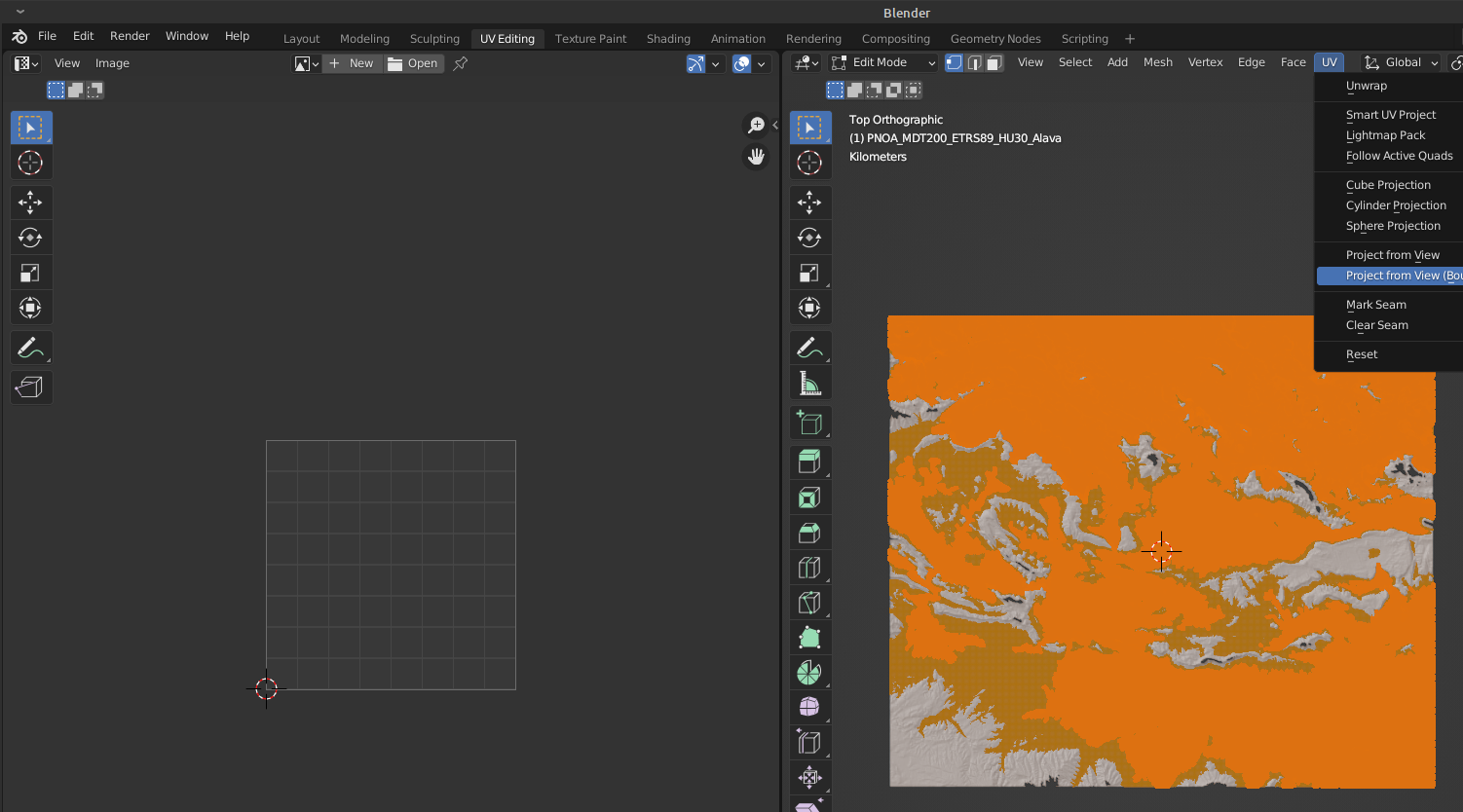
Now move to UV Editing tab.
Select the terrain layer on the right window, enter Edit Mode, and "Select all" faces (Ctrl+A). You should see it orange as below and make sure you are in "Top" view (press number 7).
Click on "UV" tools in the top menu and project the terrain layer with "Project from View (bounds)". This makes it fit the image extent.
On the left window, choose the image texture to apply to the projection and see how the grid adjusts to it (try making zoom on it)
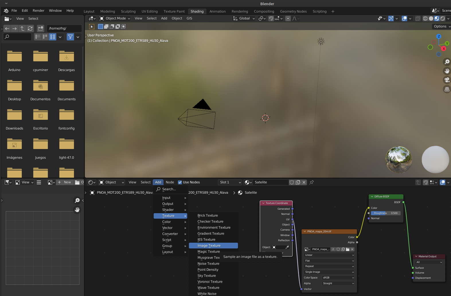
Finally, go to the Shading tab and add the element "Image Texture", choosing the right image and connecting Vector to UV and Color to Shader (just copy the image below).
If you now go to the Layout window, the model will show the satellite image perfectly adjusted.
And it's ready so you can edit and export your model, for example, for 3D printing or for a realistic Unity3D scene.
If you want to check some of the tracking that websites do while you browse, make this simple experiment:
Open the browser inspector with Ctrl+I or right click and “Inspect”
Open the “Network” tab.
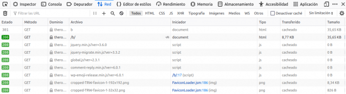
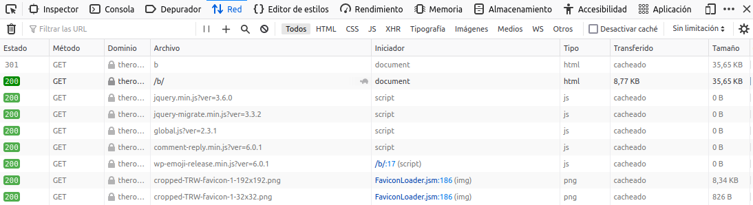
Now refresh the main page of this blog.
This is what you’ll see: just 8 files that load all what’s needed to browse this blog.
Now open any other website that you use to visit and observe the content that’s loaded.
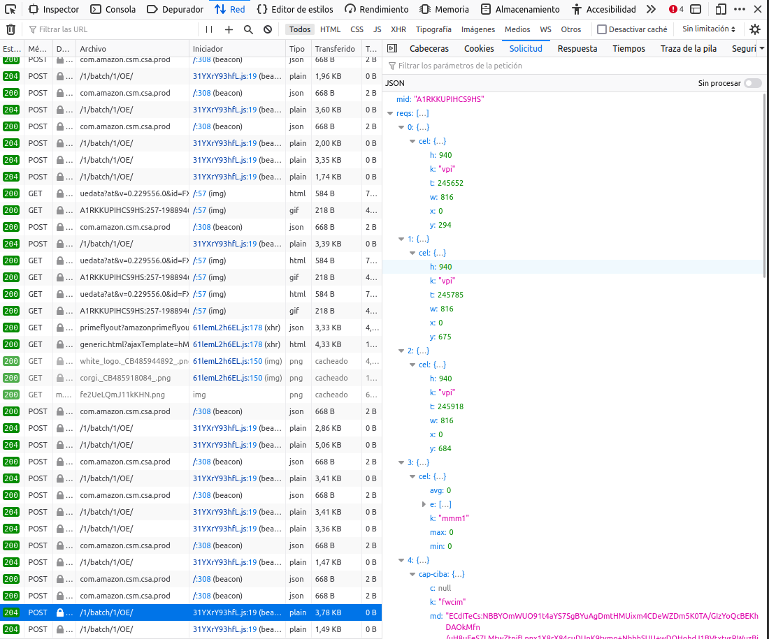
I’m going to visit amazon.es without any further interaction. Just see there’s a file at the end being created every couple of seconds /1/batch/1/OE . Now move the cursor without scrolling the window. The new files will show a variable t for the time you’ve been on the site, and coordinates x and y that show where you place the cursor. This is just an example of how tracking is used very often: where did you access the site from, what you click, what you see, where you stop, you IP, geolocation… There’s nothing of that in here.
This is only Amazon and its AWS. Google tracking shows up as its famous “analytics” or “collect” files in the Network tab as well.
It’s often said that the simplest is the best solution, in fact, you’ll see in this blog that you don’t need so many frills to publish a website. So don’t trust complicated sites, with never-ending “partners” lists and with Google Analytics or Amazon Web Services.
With a quick calibration you can use any analog pin as a tactile sensor. Despite there are a few libraries about this, you really just need a couple of function, so let’s get on with it!
Content
Components
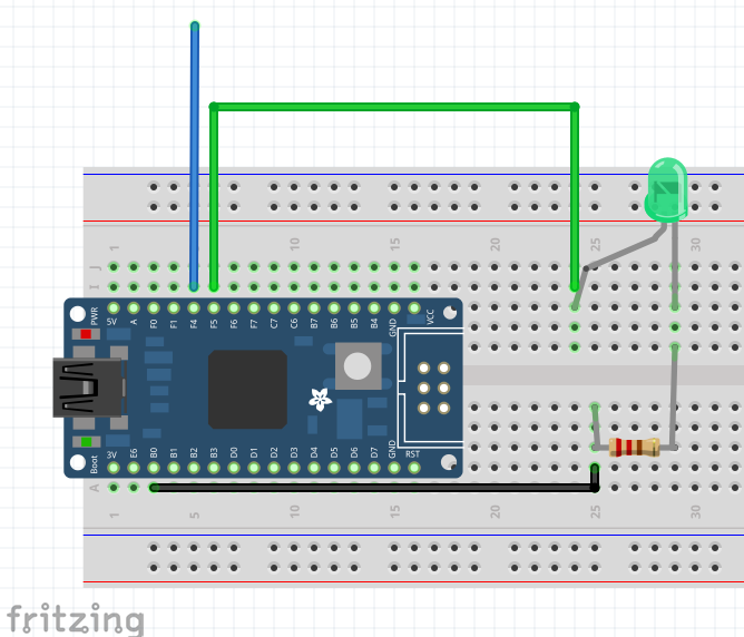
For this project I am using these simple components:
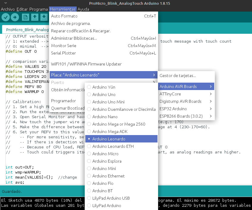
It states "ProMicro" but it can really be used with any compatible microcontroller board. You just need to select your board in the board manager.
The Pro Micro runs a ATMega32u4, which is compatible with the Arduino Leonardo board.
With this config, compile the script and upload to the board.
Result
Open the Serial Monitor, which should show blank as the debugging text is set to minimum by default.
Now we touch the free pin of the jumper wire and see how the led lights, and how the "touch" is detected in the Serial Monitor.
You'll also see that the script accumulates "touches" so this can be used in other programs.
The code
Briefly this is what the program does:
During setup(), start serial communication, activate led pin and fill-up the analog readings array with setTouch (Reads 20 values by default).
void setup() {
  // initialize serial communication at 115200 bits per second:
  Serial.begin(115200);
  //enable LED pin
  pinMode(LP,OUTPUT);
  setTouch(TP);
}
Next we run the loop() function, where the readings are updated at the start of each loop.
setTouch(TP);
//------loop continues------//
void setTouch(int tp){
  //fill up the array
  for(int a=0;a<VALUES;a++){
    mean[a]=analogRead(tp);
    delay(10);
  }
}
Check if debugging is minimal or extended, and run the main function (the only difference is the amount of debugging messages).
Calculates the difference between new reading and average,
If the difference is bigger than the REFV voltage drop value: "touch" is identified, it's printed in Serial Monitor, touch counter is increased and led is lit.
Restore average to 0, turn led off and return "touch" variable.
int minimal(int tp){
  //start reading values
  for(int i=0;i<VALUES;i++){
    //get average of array
    for(int j=0;j<VALUES;j++){
      avg+=mean[j];
    }

    avg=avg/VALUES;

    //read current value
    fin=analogRead(tp);

    //compare average with current value
    if((avg-fin)>REFV){
      Serial.println("----------  T   O    U    C    H  ----------");
      //increase counter
      touch++;
      //print touch count
      Serial.print("T: ");
      Serial.println(touch);
      //light led
      ledON(LP);
      //wait 1 second after touch detected
      delay(1000);
    }
    //restart counter
    avg=0;
    //restart led
    ledOFF(LP);
    delay(VALINTERVAL);
  }
  return touch;
}
After this the loop is restarted, going back to point 2.
Other configurations
The script includes different configuration variables that we find under the '#define's:
OUT: defines the amount of debugging text. Value 0: minimal; Value 1: extended.
VALUES: analog readings array size.
TOUCHPIN: define the analog pin number used for touch.
LEDPIN: define the pin number used for led.
VALINTERVAL: evaluation interval in milliseconds.
REFV: voltage drop value (in millivolts) which identifies a "touch".
// OUTPUT verbosity
// 1: extended --> Prints ADC array, mean value, touch count and touch message with touch count
// 0: minimal  --> Prints touch message with touch count

#define OUT 0

// comparison variables
#define VALUES 20       //values for mean array
#define TOUCHPIN 3      //touch pin
#define LEDPIN 20       //led pin
#define VALINTERVAL 100 //evaluation interval
#define REFV 80         //reference voltage drop in mV
Calibration
Changing the configuration you can calibrate the script for different boards. From what I've tested, this is a good sequence:
Set a high REFV, for example 100.
Run the extended script with OUT 1
Open Serial Monitor and have a look at the average values for a while (e.g.: 230)
Now touch the jumper wire and see what the values are now (e.g.: 170)
Make the difference between the average at 3. and the average at 4 (230-170=60).
Set your REFV to this value (60) and play around it.
For more sensitivity, set it a bit lower (50)
If there is detection with no touch, increase it (80)
Because of CPU load, REFV value can vary if OUT 1 or OUT 0
Found it useful? Any doubts? Leave your comment on 🐦 Twitter!
If you’ve used desktop GIS software, you will be surprised that many geospatial tools are also available to use in your web maps using a free and open-source javascript library.
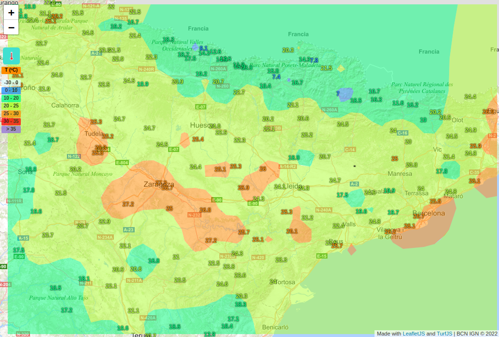
Today I show you TurfJS. Press the button 🌤 in the map below and see one of many possibilities: inverse distance weighting or IDW.
Content
Installation
TurfJS hosts a practical website explaining all available functions, as well as the initial setup:
markers.forEach(function(m){
    var marker=L.marker([m.lat, m.lon]).addTo(map);
    marker.bindTooltip("<b>"+m.name+"</b><br>"+m.dato).openTooltip();
});

//WE ADDED A SINGLE MARKER LIKE THIS ON LEAFLET
//var marker = L.marker([25.77, -80.13]).addTo(map);
//marker.bindTooltip("<b>Estacion1</b><br>m.dato").openTooltip();
//empty points array
var points=[];

//loop to fill the array with data
markers.forEach(function(m){
    points.push(turf.point([m.lon, m.lat],{name: m.name, dato: m.dato}));
});

//convert to Turf featureCollection
points=turf.featureCollection(points);
TIP! Note that Turf taked coordinates as longitude-latitude, instead of the usual latitude-longitude!
Define interpolation options, having the following:
gridType: or cell shape
points
square
hex
triangle
property: field that contains the interpolation values.
units: spatial units used in the interpolation:
miles
kilometers
radians
degrees
weight: power used in the inverse distance weighting, usually 2, although higher values will make a smoother result.
//interpolation options: rectangular grid using 'dato' variable in kilometers using the power of 2

var options = {gridType: 'square', property: 'dato', units: 'kilometers', weight: 2};
Finally, generate the interpolated grid and add it to the map, being the numeric value the cell size of the grid (0.5 Km):
//create Turf grid
var malla=turf.interpolate(points, 0.5, options);

//add to Leaflet
L.geoJSON(malla).addTo(map);
Generating this result (nothing conclusive):
Format grid and show values
Seems not, but the interpolation is done, it's just shown incorrectly.
I'll add a color ramp to represent data, and also show values when hovering the cells. Let's modify the Leaflet geoJSON object properties for this:
style: function to modify object style, according to its value.
onEachFeature: function added to each object to interact with it.
TIP! Always download files from the official source published bh me, the author. DONT execute files shared by third parties. Javascript code can de easily manipulated to run malicious activities.
Description
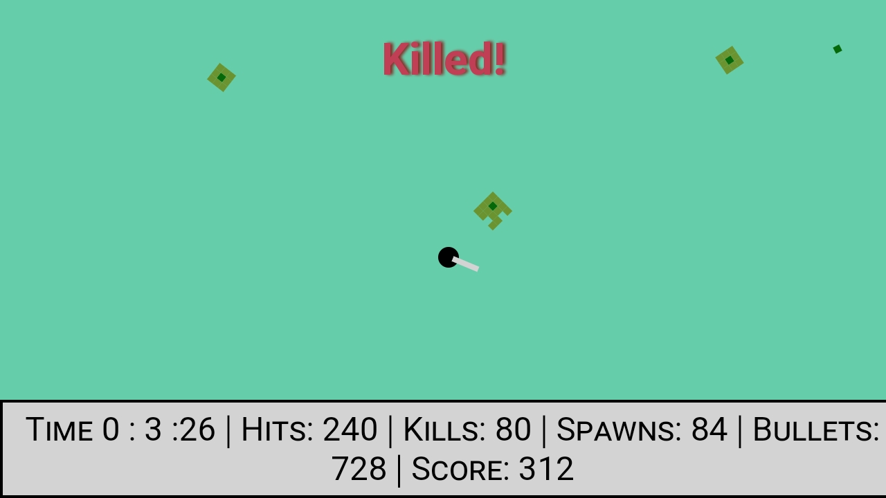
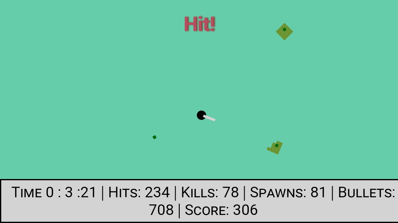
You are a survivor with unlimited ammo surrounded by zombies, how long can you survive?
Randomness will make every game unique: zombie enemies are randomly generated in random border locations with random attributes (speed and level).
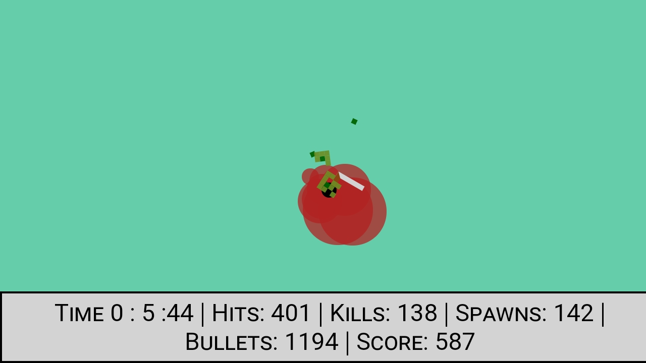
There are 4 zombie levels, making them bigger and harder to kill (1×1, 2×2, 3×3, 4×4).
The game is infinite as long as you can keep up killing zombies.
Wasting ammo reduces your score though, so make accurate shots!
Game instructions
Click or touch a point in the map to shoot to that place.
Every bullet used deduces 1 point (-1).
Shooting body parts (light green) adds 1 point (+1).
Shooting in the head (dark green) adds 10 points (+10).
Survival time will also add score points in the future.
Let’s now pay attention to the detail of the API and how to access all the available data.
Content
API access
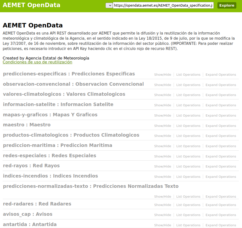
To use the API we need an API key. Go to the AEMET OpenData webpage and click on "Solicitar" to request it.
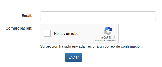
Next we'll be asked for an email address where the key will be sent.
You'll receive a first confirmation email, and then a second email with the access key. Let's copy it and keep moving.
Documentation and examples
Get back to AEMET OpenData and into the developer's section "Acceso Desarrolladores".
We're interested in the dynamic documentation, which shows all the data requests available that we can try live.
Click on each topic to display the syntax for every data request.
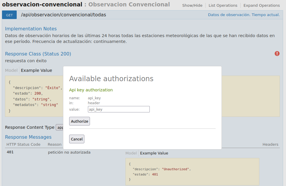
Click on observación-convencional and then /api/observacion/convencional/todas.
Now click on the red sign on the right, where you'll paste and authorize the API key.
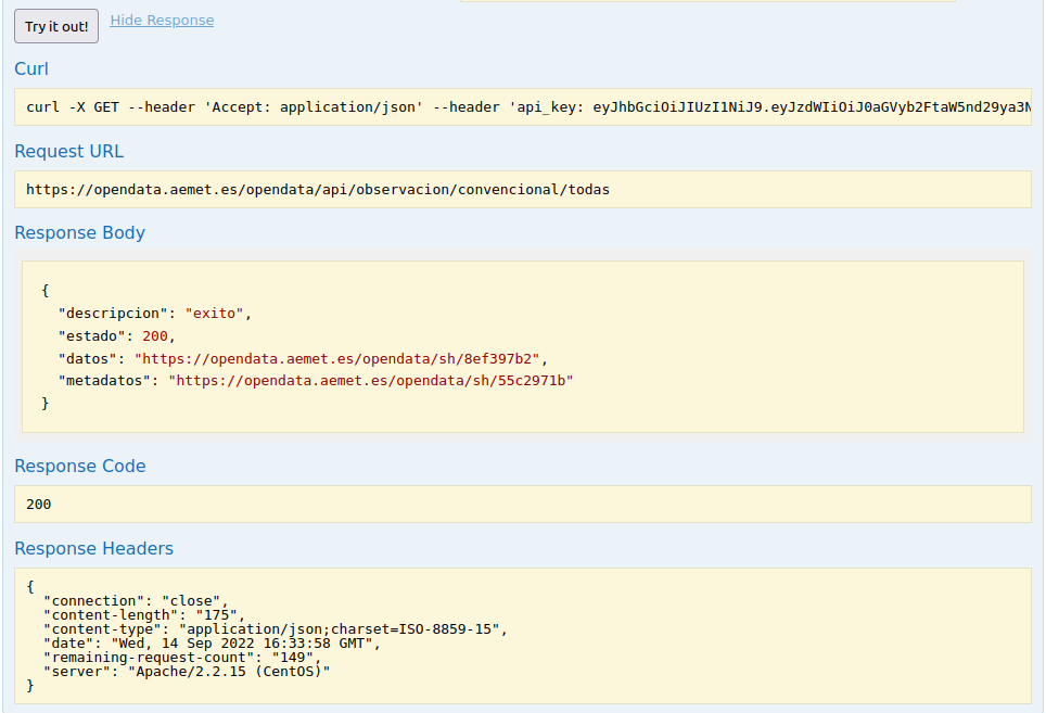
Now press the Try it out! button and you'll get:
a curl request example
the request URL
the body, code and headers of the response
If we open the URL inside the "datos" field we'll see the full list of data for all the stations. A JSON lot like this:
Loading...
The main fields are the following:
idema: station ID or code.
lat and lon: latitude and longitude coordinates.
alt: station altitude.
fint: data interval date.
prec: precipitation in this period.
vv: wind speed in the station.
ta: ambience temperature in the station.
Data request using javascript
HTML structure
I'll develop an example to access the data and make use of them.
I'll simply create a .html document with a request button, a text line and a request function:
Click the button to request data
<html>
<body>
<button id="solicitud" onclick="solicitar()">Request</button>
<p id="texto">Click the button to request data</p>
</body>
<script>
function solicitar(){
document.getElementById("texto").innerHTML="I didn't program that yet..";
}
</script>
</html>
TIP! Copy and paste the code above in a text document with .html extension and open it in your browser.
HTTP request
We'll do the data request in javascript using the XMLHttpRequest object. The example from w3schools is really simple:
As we saw in the dynamic documentation, after doing the request, we got a link to the data, which is another request, no we need to nest two requests like this:
<script>
function solicitar(){
// Define loading message
document.getElementById("texto").innerHTML="Cargando datos...";
// Define API Key
var AK=tUApiKey;
// Define request URLs
var URL1="https://opendata.aemet.es/opendata/api/observacion/convencional/todas";
var URL2="";

// Create XMLHttpRequest objects
const xhttp1 = new XMLHttpRequest();
const xhttp2 = new XMLHttpRequest();

// Define response function for the first request:
// We want to access te "datos" URL
xhttp1.onload = function() {
  // 1º Parse the response to JSON:
  URL2=JSON.parse(this.responseText);
  // 2º Get the "datos" field:
  URL2=URL2.datos;
  // 3º Make the new request:
  xhttp2.open("GET", URL2);
  xhttp2.send();
}

// Define response function for the second request:
// We'll modify the text line with some information in the data
xhttp2.onload = function() {
  // 1º Parse the response to JSON (much better to work with):
  var datos=JSON.parse(this.responseText);

  // 2º Get the length of the JSON data
  // This is equivalent to the individual hourly entries per stations
  var registros=datos.length;

  // 3º Get first entry date.
  // We'll format it as it's in ISO standard
  var fechaini=datos[0].fint;
  fechaini=new Date(fechaini+"Z");
  fechaini=fechaini.toLocaleDateString()+" "+fechaini.toLocaleTimeString();

  // 4º Get last entry date.
  // We'll format in the same way
  var fechafin=datos[(datos.length-1)].fint;
  fechafin=new Date(fechaini+"Z");
  fechafin=fechafin.toLocaleDateString()+" "+fechafin.toLocaleTimeString();

  // 5º Merge it all and display in the text line
  document.getElementById("texto").innerHTML="Se han descargado <b>"+registros+"</b> registros desde el <b>"+fechaini+"</b> hasta el <b>"+fechafin+"</b>. <a href='"+URL2+"' target='_blank'>Ver todos los datos.</a>";
}

// Send the first request
xhttp1.open("GET", URL1+"/?api_key="+AK);
xhttp1.send();

}
</script>
Let's see the result below:
Click the button to request data
And done! This way you can obtain coordinates and values for different metheorological stations from AEMET and drop them in a table or web map like we've seen for Leaflet here.
The usual way to see and work with these files is using a GIS software like QGIS or ArcGIS, but how can we make this friendly to standard users? Wouldn’t it be better seen directly in 3D and visit the place virtually?
At this point is where I found CesiumJS: a 3D map viewer styling [G] Earth but open-source, free and highly customizable to make your own projects.
CesiumJS demo viewer of the new Tajogaite terrain with IDE Canarias satellite imagery. Click on the map to interact or open the full version.
Content
Create a Cesium ion account
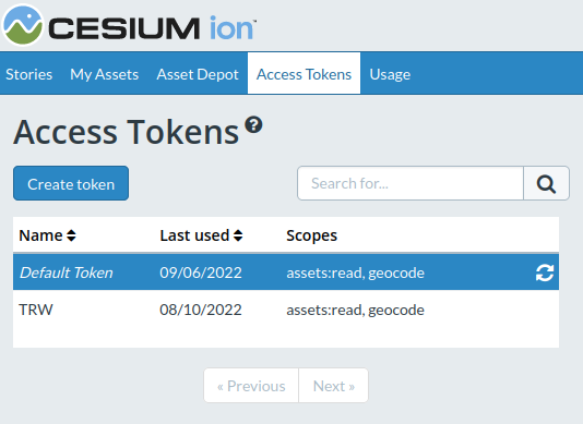
To use CesiumJS you need to register an account in order to obtain an Access Token.
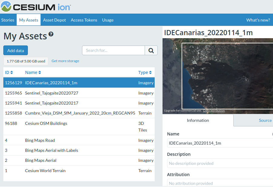
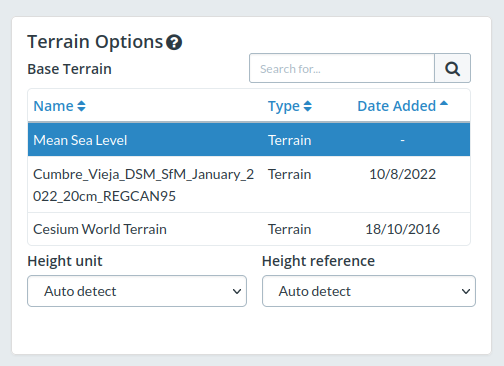
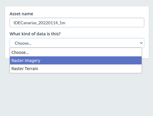
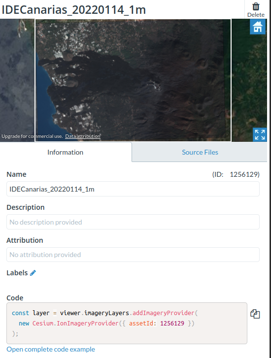
Registering, we can also upload our own files to customize our 3D map creations. In my case you can see that I uploaded the Digital Surface Model and imagery of the viewer. I drop the links in case you want to use the same files:
TIP! You can use the WMS service in your GIS software to extract the imagery, or download the one I use in this example (270 MB with 1m resolution)
Include CesiumJS in your web.
To use CesiumJS we configure a .html file as usual.
In this case, I'll copy the code directly from their quickstart example as it is only about 25 lines:
As you see, the main parts are:
links to CesiumJS libraries in the <head>
a <div> element with id "cesiumContainer" inside the <body>
the Access Token as variable Cesium.Ion.defaultAccessToken. Introduce yours here.
a "viewer" variable
the initial viewer configuration, specifying initial coordinates and X, Z angles.
<!DOCTYPE html>
<html lang="en">
<head>
  <meta charset="utf-8">
  <!-- Include the CesiumJS JavaScript and CSS files -->
  <script src="https://cesium.com/downloads/cesiumjs/releases/1.97/Build/Cesium/Cesium.js"></script>
  <link href="https://cesium.com/downloads/cesiumjs/releases/1.97/Build/Cesium/Widgets/widgets.css" rel="stylesheet">
</head>
<body>
  <div id="cesiumContainer"></div>
  <script>
    // Your access token can be found at: https://cesium.com/ion/tokens.
    // This is the default access token from your ion account
    Cesium.Ion.defaultAccessToken = 'eyJhbGciOiJIUzI1NiIsInR5cCI6IkpXVCJ9.eyJqdGkiOiI1MTYwNGM0Yi1iYzlkLTRkMTUtOGQyOS04YjQxNmUwZDQ0YjkiLCJpZCI6MTA0Mjc3LCJpYXQiOjE2NjAxMDk4MzR9.syNWeKPLWA2eMrEh4K9hvkyp1oGdbLMaL0Ozk1kaksk';
    // Initialize the Cesium Viewer in the HTML element with the `cesiumContainer` ID.
    const viewer = new Cesium.Viewer('cesiumContainer', {
      terrainProvider: Cesium.createWorldTerrain()
    });
    // Add Cesium OSM Buildings, a global 3D buildings layer.
    const buildingTileset = viewer.scene.primitives.add(Cesium.createOsmBuildings());
    // Fly the camera to San Francisco at the given longitude, latitude, and height.
    viewer.camera.flyTo({
      destination : Cesium.Cartesian3.fromDegrees(-122.4175, 37.655, 400),
      orientation : {
        heading : Cesium.Math.toRadians(0.0),
        pitch : Cesium.Math.toRadians(-15.0),
      }
    });
  </script>
 </div>
</body>
</html>
<html lang="en">
<head>
<meta charset="utf-8">
<script src="https://cesium.com/downloads/cesiumjs/releases/1.96/Build/Cesium/Cesium.js"></script>
<link href="https://cesium.com/downloads/cesiumjs/releases/1.96/Build/Cesium/Widgets/widgets.css" rel="stylesheet">
</head>
<body style="margin:0;width:100vw;height:100vh;">
<div style="height:100%;" id="cesiumContainer"></div>
<script>
// Your access token can be found at: https://cesium.com/ion/tokens.
// Replace `your_access_token` with your Cesium ion access token.
Cesium.Ion.defaultAccessToken = 'eyJhbGciOiJIUzI1NiIsInR5cCI6IkpXVCJ9.eyJqdGkiOiI1MTYwNGM0Yi1iYzlkLTRkMTUtOGQyOS04YjQxNmUwZDQ0YjkiLCJpZCI6MTA0Mjc3LCJpYXQiOjE2NjAxMDk4MzR9.syNWeKPLWA2eMrEh4K9hvkyp1oGdbLMaL0Ozk1kaksk';
// Initialize the Cesium Viewer in the HTML element with the `cesiumContainer` ID.
const viewer = new Cesium.Viewer('cesiumContainer', {
//terrainProvider: Cesium.createWorldTerrain()//terreno original
terrainProvider: new Cesium.CesiumTerrainProvider({//terreno modificado
url: Cesium.IonResource.fromAssetId(1255858),
}),
});
// Esconder widgest inferiores
viewer.timeline.container.style.visibility = "hidden";
viewer.animation.container.style.visibility = "hidden";
// Add Sentinel2 imagery
const layer = viewer.imageryLayers.addImageryProvider(
new Cesium.IonImageryProvider({ assetId: 1256129 })
);
// Add Cesium OSM Buildings, a global 3D buildings layer.
const buildingTileset = viewer.scene.primitives.add(Cesium.createOsmBuildings());
// Fly the camera to San Francisco at the given longitude, latitude, and height.
viewer.camera.flyTo({
    destination : Cesium.Cartesian3.fromDegrees(-17.8195, 28.6052, 3000),
    orientation : {
    heading : Cesium.Math.toRadians(-85.0),
    pitch : Cesium.Math.toRadians(-30.0),
    }
});
</script>
</div>
</html>
And that's it! You can create tons of immersive web apps with detailed terrains better than the standard ones.
Where else can you use CesiumJS? Tell it on Twitter 🐦
One of my latest projects is a notes app that is hosted in my server so I can stop using [G] Notes.
An interesting feature that I am including is Rich Text Editor, a rich javascript library in the form of user interface to format HTML text of any web form.
It’s open source, free for personal use, and very simple to use. A true win-win that I’m showing you today.
Content
License
I said Rich Text Editor is free, and it is for a non-commercial use.
It's important that you read their pricing page to understand the limitations of the free license:
1 developer
1 domain
5 active users
In my case, I installed Rich Text Editor in this server that hosts the blog, and it's been restricted with php so it's only accessible from the same domain.
TIP! Do NOT host the files anywhere accessible for anyone (like a public server), as you might lead to a license break, being forced to pay a standard license or retiring your app.
Anyway, commercial licenses are one-off payments and it might be worth getting one if you're going to give it plenty of use.
Installation
Using Rich Text Editor is very simple and it's explained in their document page.
To install Rich Text Editor you only need to download the files from their website in a local folder or in your web server.
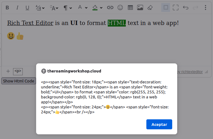
One basic funcionality is to capture the full HTML code for the text that we have been editing. That's what the button at the bottom does, using the getHTMLcode():
<button onclick="alert(editor1.getHTMLCode())">Show Html Code</button>
Uses
As stated previously, I'll be using this library as an editor for a notes app that will be hosted in my server.
The editor will let me easily add nice formatting to the notes and save them with the full format code.
Here you have a demo of how the interface is looking, although there are no functions enabled so far.
Other applications where you can use this editor are self-made forums, user forms, comments boxes or any text-box where a user needs to input text in your web app.
I hope you found this useful as I did and give it good use. Any doubts or comments, drop them on Twitter 🐦 See you soon!