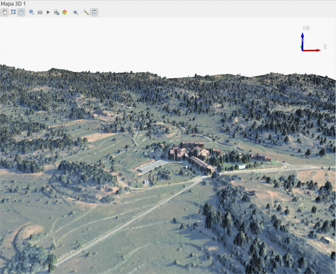
After a few posts about the use of satellite information, let’s see how to bring it (almost) all together in a practical and impacting example. And it’s given the latest wildfires occurred in Spain that they’ve called my attention as I could not imagine how brutal they have been (although nothing compared to the ones in Chile, Australia or USA). But let’s do the exercise without spending too much GB in geographical information.
What I want is to show the extent of the fire occurred in Asturias in March, but also to show the impact removing the trees affected by the flames. Let’s do it!
Download data
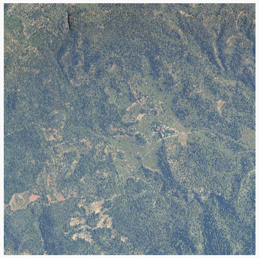
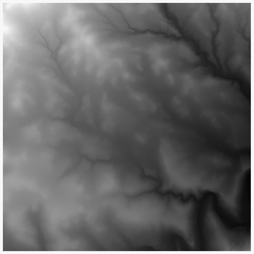
I will need a Digital Surface Model (which includes trees and structures), an orthophoto taken during the fire, and a Digital Terrain Model (which has been taken away trees and structures) to replace the areas affected by the fire.
1. Terrain models
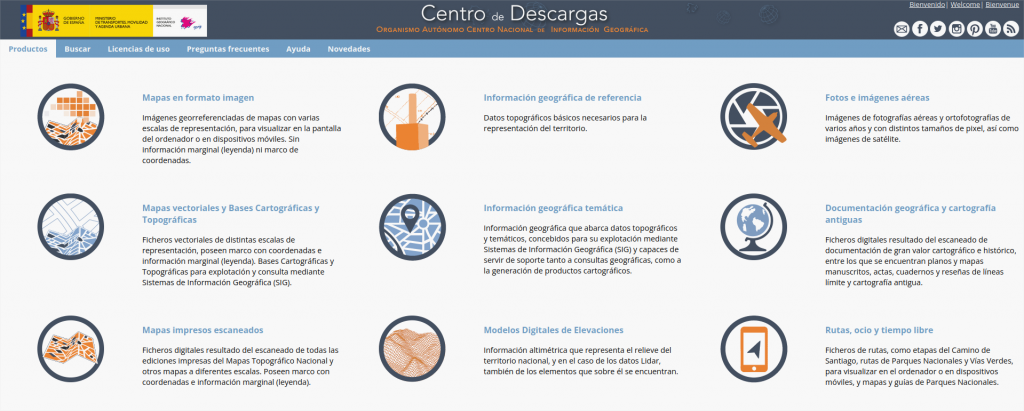
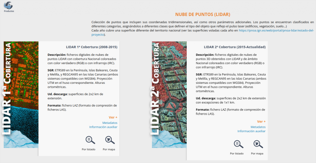
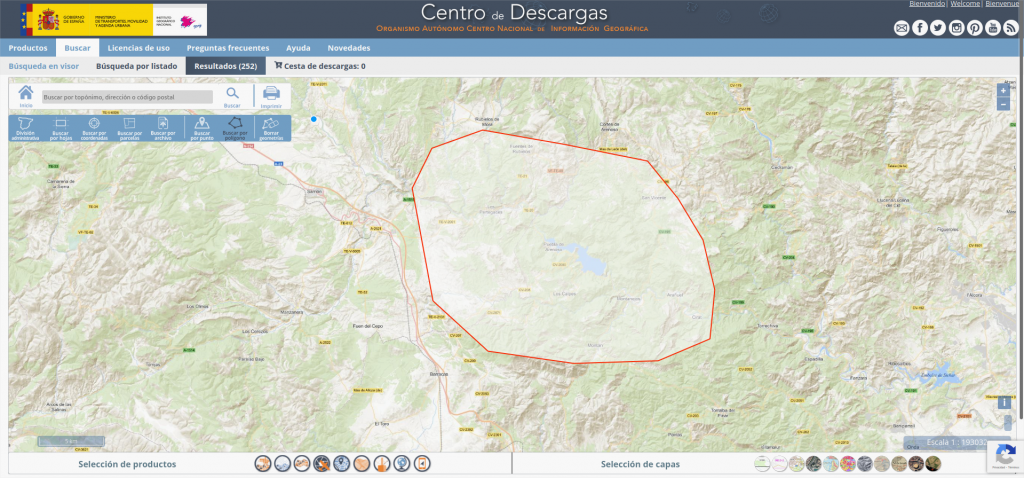
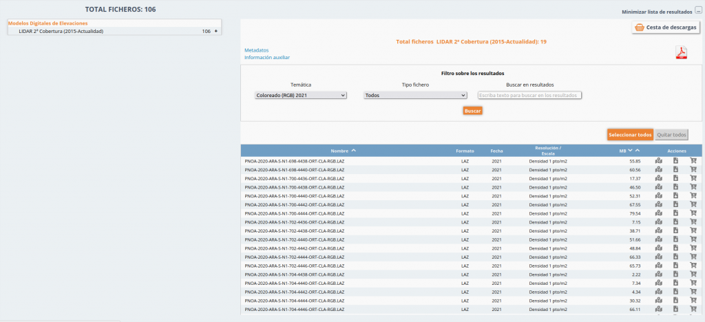
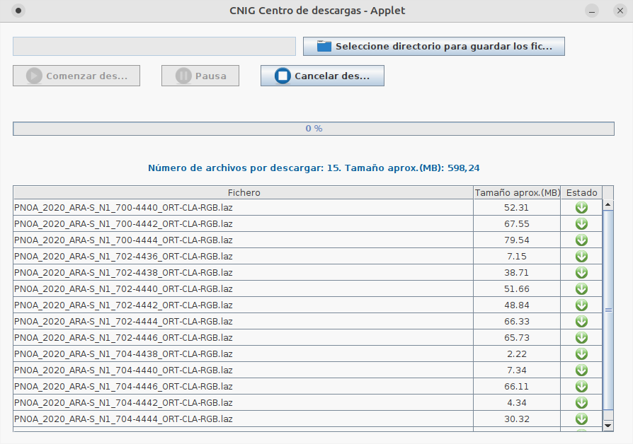
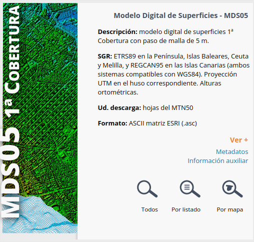
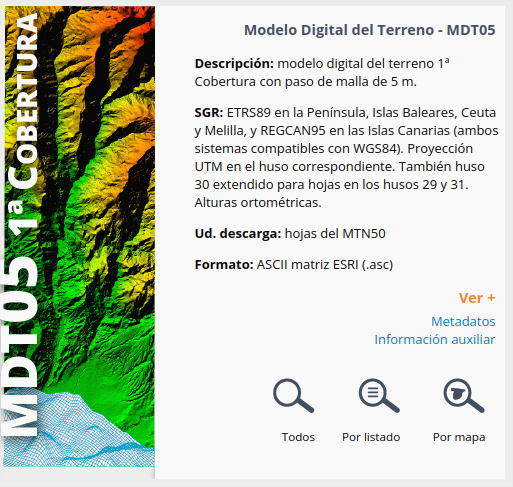
I'm going to use the great models from Spanish IGN, downloading the products MDS5 and MDT5 for the area.
http://centrodedescargas.cnig.es/CentroDescargas/index.jsp
2. Orthophotos
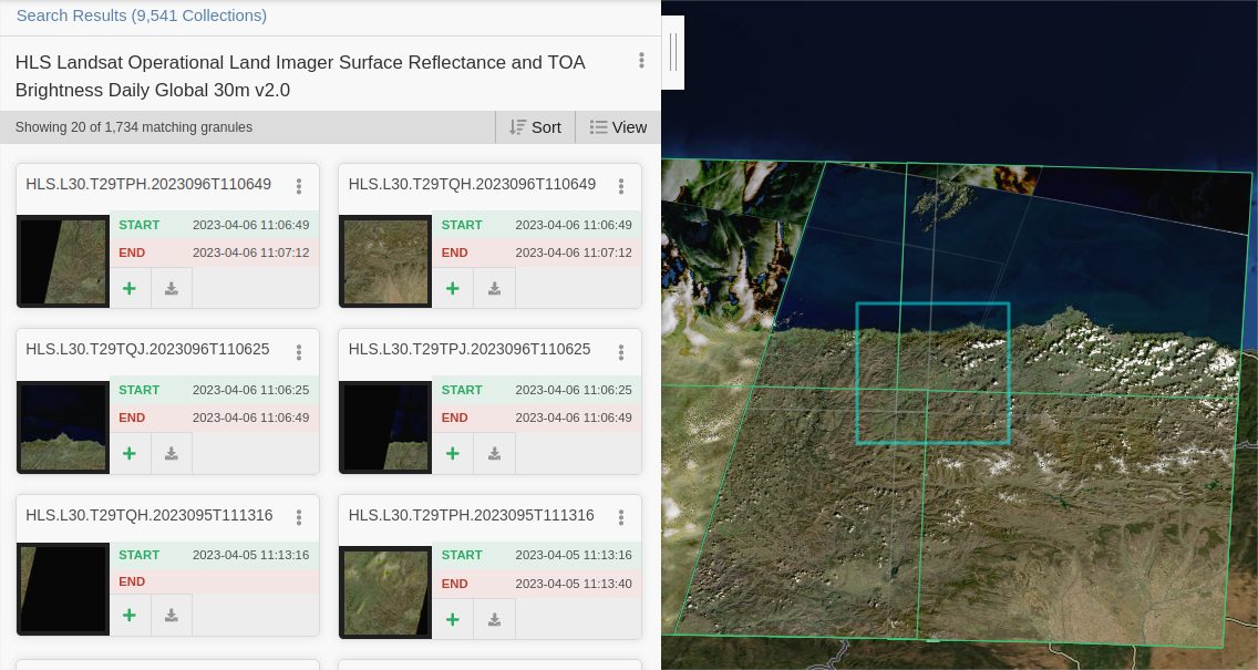
As per satellite imagery, I decided to go for Landsat this time, as it had a clearer view during the last days of the fire.
I will be using the images taken on 17th February 2023 (before the fire) and 6th April 2023 (yet in the last days).
https://search.earthdata.nasa.gov
Process satellite imagery
We'll use the process i.group from GRASS in QGIS to group the different bands captured by the satellite in a single RGB raster, as we saw in this previous post:
You'll have to do it for every region downloaded, four in my case, that will be joint later using Build virtual raster
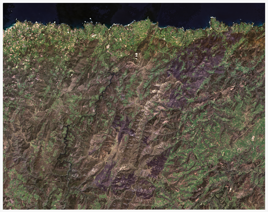
1. True color image (TCI)
Combine bands 4, 3, 2.
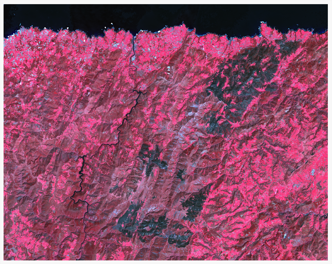
2. False color image
Combine bands 5, 4, 3.
3. Color adjustment
To get a better result, you can adjust the minimum and maximum values considered in each band composing the image. These values are found in the Histogram inside the layer properties.
here you have the values I used for the pictures above::
| Band | TCI min | TCI max | FC min | FC max |
|---|---|---|---|---|
| 1 Red | -100 | 1500 | -50 | 4000 |
| 2 Green | 0 | 1500 | -100 | 2000 |
| 3 Blue | -10 | 1200 | 0 | 1200 |
Fire extent
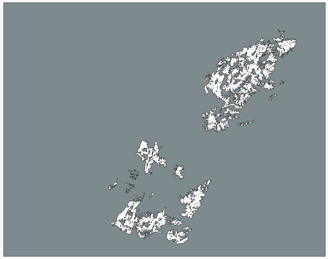
As you can see, the false color image shows a clear extension of the fire. We'll generate a polygon covering the extent of the fire with it.
First, let's query the values in Band 1 (red) which offers a good contrast for values in the area of the fire. They are in the range 300-1300.

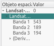
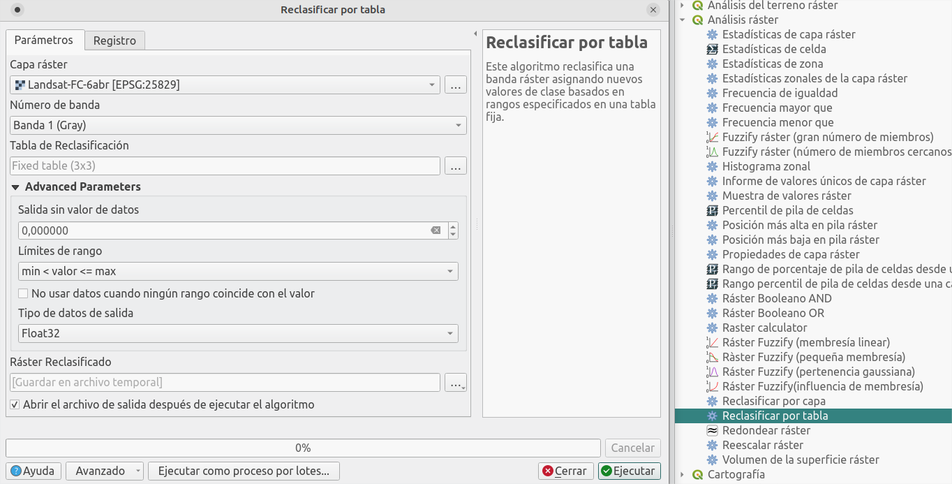
Using the process Reclassify by table, we'll assign value 1 to the cells inside this range, and value 0 to the rest.
Vectorize the result with process Poligonize and, following the satellite imagery, select those polygons in the fire area.
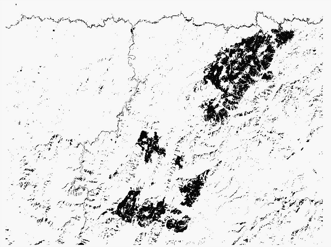
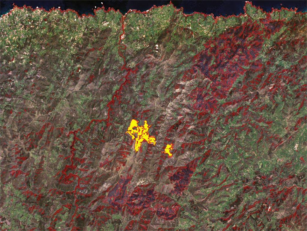
Use the tool Dissolve to merge all the polygons in one element; then Smooth to round the corners slightly.
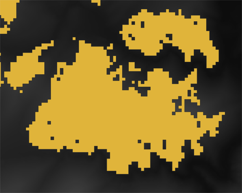
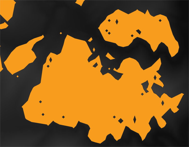
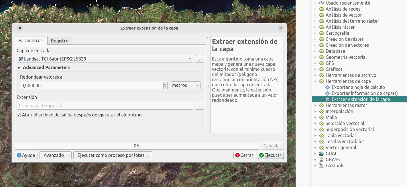
Let's now get the inverse. Extract by extent using the Landsat layer, then use Difference with the fire polygon.
Process terrain
1. Combine terrain data
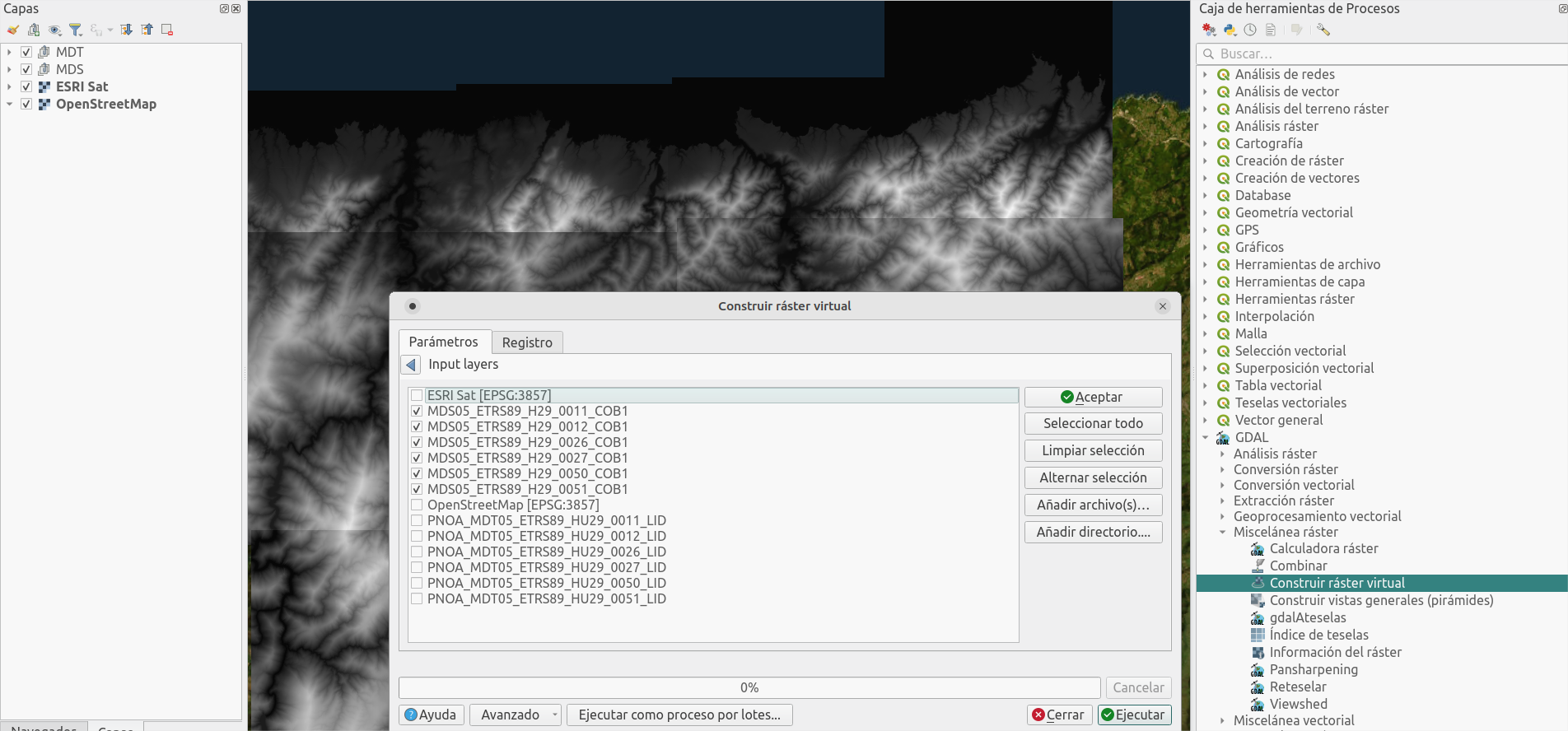
Join the same type model files in one (one for the DSM, and another one for the DTM). Use process Build virtual raster
2. Extract terrain data
Extract the data of interest in each model:
- From the DSM extract the surface affected by the fire, so you'll remove all the surface in it.
- Do the opposite with the DTM: keep the terrain (without trees) in the fire area, so it will fill the gaps in the other model.
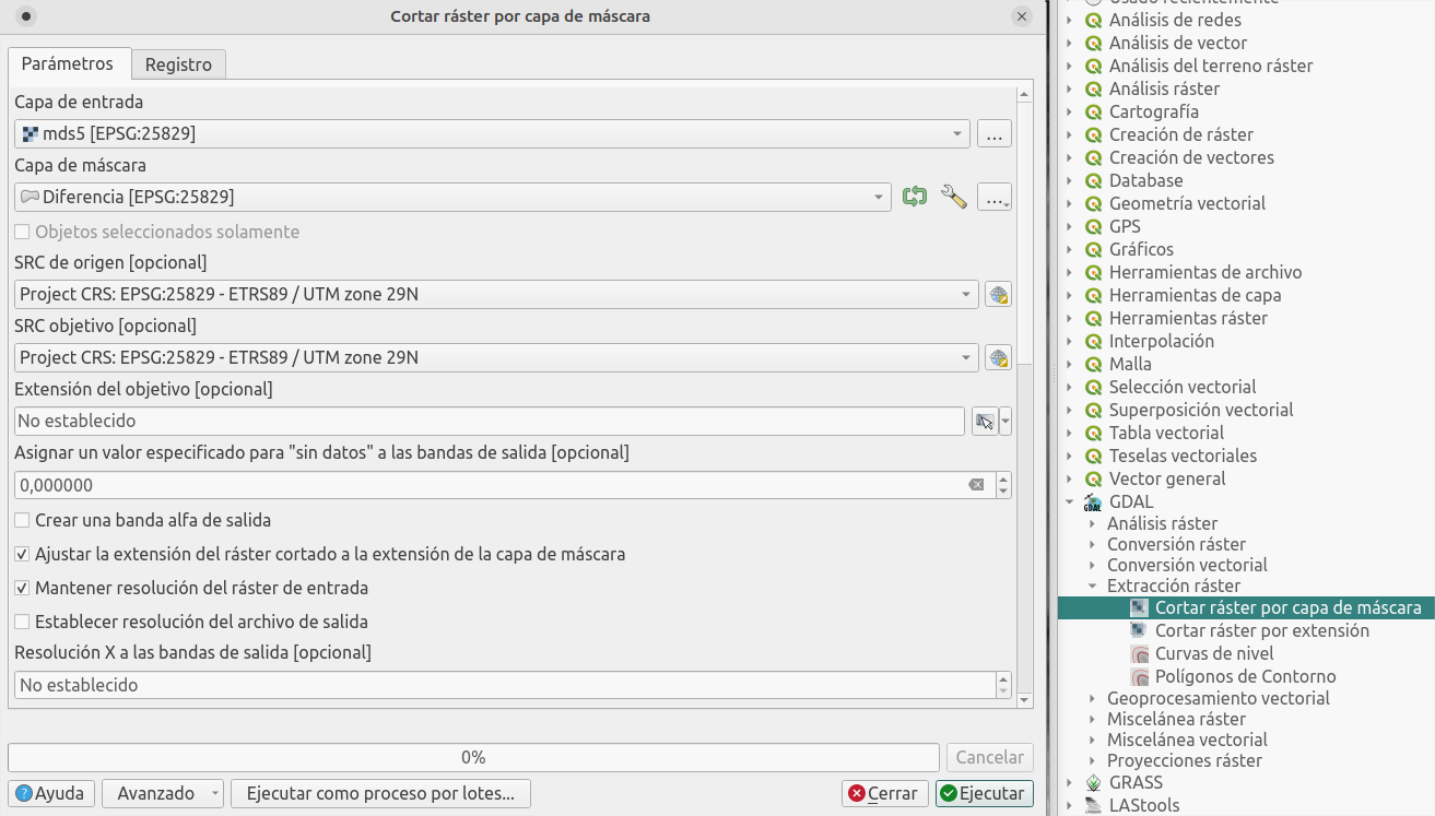
Use the process Crop raster by mask layer using the layers generated previously.
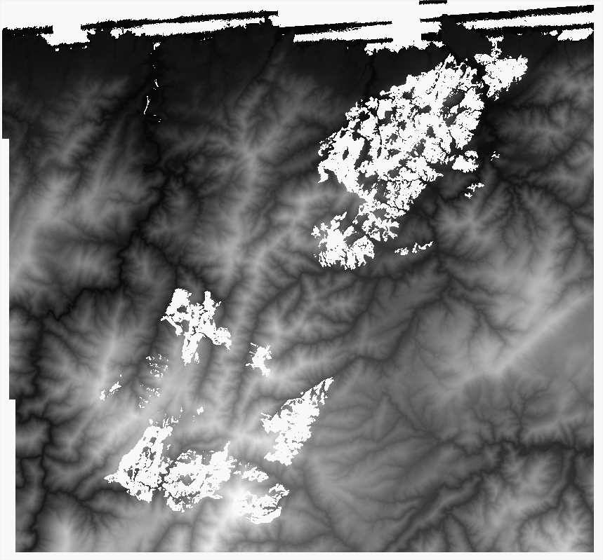
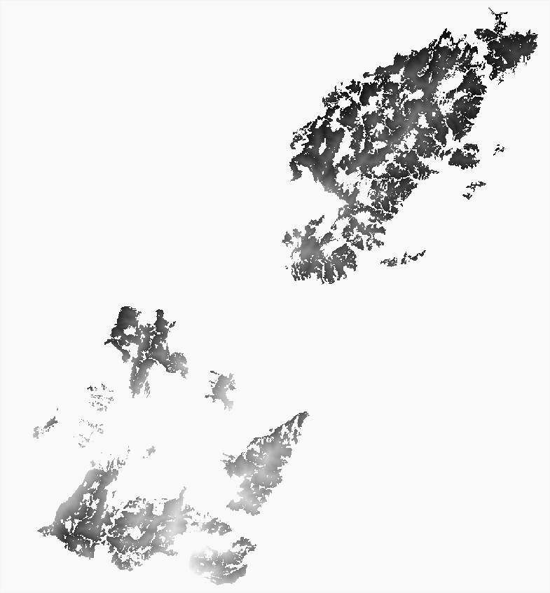
Finally join both raster layers, so they fill each others' gaps, using Build virtual raster.
Bring it to life with Cesium JS
You should already have a surface model without trees in the fire area, but let's try to explore it in an interactive way.
I showed a similar example, using a custom Digital Terrain Model, as well as a recent satellite image, for the Tajogaite volcano in La Palma:
https://theroamingworkshop.cloud/b/1319/cesiumjs-el-visor-gratuito-de-mapas-en-3d-para-tu-web/
In this case I'll use Cesium JS again to interact easily with the map (follow the post linked above to see how to upload your custom files to the Cesium JS viewer).
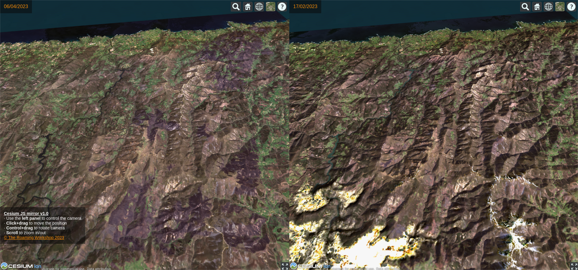
For this purpose, I created a split-screen viewer (using two separate instances of Cesium JS) to show the before and after picture of the fire. Here you have a preview:
https://theroamingworkshop.cloud/demos/cesiumJSmirror/
I hope you liked it! here you have the full code and a link to github, where you can download it directly. And remember, share your doubts or comments on twitter!
<html lang="en">
<head>
<meta charset="utf-8">
<title>Cesium JS mirror v1.0</title>
<script src="https://cesium.com/downloads/cesiumjs/releases/1.96/Build/Cesium/Cesium.js"></script>
<link href="https://cesium.com/downloads/cesiumjs/releases/1.96/Build/Cesium/Widgets/widgets.css" rel="stylesheet">
</head>
<body style="margin:0;width:100vw;height:100vh;display:flex;flex-direction:row;font-family:Arial">
<div style="height:100%;width:50%;" id="cesiumContainer1">
	<span style="display:block;position:absolute;z-Index:1001;top:0;background-color: rgba(0, 0, 0, 0.5);color:darkorange;padding:13px">06/04/2023</span>
</div>
<div style="height:100%;width:50%;background-color:black;" id="cesiumContainer2">
	<span style="display:block;position:absolute;z-Index:1001;top:0;background-color: rgba(0, 0, 0, 0.5);color:darkorange;padding:13px">17/02/2023</span>
	<span style="display:block;position:absolute;z-Index:1001;bottom:10%;right:0;background-color: rgba(0, 0, 0, 0.5);color:white;padding:13px;font-size:14px;user-select:none;">
		<b><u>Cesium JS mirror v1.0</u></b><br>
		· Use the <b>left panel</b> to control the camera<br>
		· <b>Click+drag</b> to move the position<br>
		· <b>Control+drag</b> to rotate camera<br>
		· <b>Scroll</b> to zoom in/out<br>
		<span><a style="color:darkorange" href="https://theroamingworkshop.cloud" target="_blank">© The Roaming Workshop <span id="y"></span></a></span>
    </span>
</div>
<script>
	// INSERT ACCESS TOKEN
    // Your access token can be found at: https://cesium.com/ion/tokens.
    // Replace `your_access_token` with your Cesium ion access token.

    Cesium.Ion.defaultAccessToken = 'your_access_token';

	// Invoke LEFT view
    // Initialize the Cesium Viewer in the HTML element with the `cesiumContainer` ID.

    const viewerL = new Cesium.Viewer('cesiumContainer1', {
		terrainProvider: new Cesium.CesiumTerrainProvider({
			url: Cesium.IonResource.fromAssetId(1640615),//get your asset ID from "My Assets" menu
		}),
		baseLayerPicker: false,
		infoBox: false,
    });

	// Add Landsat imagery
	const layerL = viewerL.imageryLayers.addImageryProvider(
	  new Cesium.IonImageryProvider({ assetId: 1640455 })//get your asset ID from "My Assets" menu
	);

	// Hide bottom widgets
	viewerL.timeline.container.style.visibility = "hidden";
	viewerL.animation.container.style.visibility = "hidden";

    // Fly the camera at the given longitude, latitude, and height.
    viewerL.camera.flyTo({
      destination : Cesium.Cartesian3.fromDegrees(-6.7200, 43.175, 6000),
      orientation : {
        heading : Cesium.Math.toRadians(15.0),
        pitch : Cesium.Math.toRadians(-20.0),
      }
    });

    // Invoke RIGHT view

    const viewerR = new Cesium.Viewer('cesiumContainer2', {
		terrainProvider: new Cesium.CesiumTerrainProvider({
			url: Cesium.IonResource.fromAssetId(1640502),//get your asset ID from "My Assets" menu
		}),
		baseLayerPicker: false,
		infoBox: false,
    });

	// Add Landsat imagery
	const layerR = viewerR.imageryLayers.addImageryProvider(
	  new Cesium.IonImageryProvider({ assetId: 1640977 })
	);

	// Hide bottom widgets
	viewerR.timeline.container.style.visibility = "hidden";
	viewerR.animation.container.style.visibility = "hidden";

    // Fly the camera at the given longitude, latitude, and height.
    viewerR.camera.flyTo({
      destination : Cesium.Cartesian3.fromDegrees(-6.7200, 43.175, 6000),
      orientation : {
        heading : Cesium.Math.toRadians(15.0),
        pitch : Cesium.Math.toRadians(-20.0),
      }
    });

    // Invoke camera tracker
    //define a loop
    var camInterval=setInterval(function(){

	},200);
    clearInterval(camInterval);

    document.onmousedown=trackCam();
    document.ondragstart=trackCam();

    //define loop function (read properties from left camera and copy to right camera)
    function trackCam(){
		camInterval=setInterval(function(){
			viewerR.camera.setView({
				destination: Cesium.Cartesian3.fromElements(
					  viewerL.camera.position.x,
					  viewerL.camera.position.y,
					  viewerL.camera.position.z
					),
				orientation: {
					direction : new Cesium.Cartesian3(
						viewerL.camera.direction.x,
						viewerL.camera.direction.y,
						viewerL.camera.direction.z),
					up : new Cesium.Cartesian3(
						viewerL.camera.up.x,
						viewerL.camera.up.y,
						viewerL.camera.up.z)
				},
			});
		},50);
	};
	//stop loop listeners (release mouse or stop scroll)
	document.onmouseup=function(){
		clearInterval(camInterval);
	};
	document.ondragend=function(){
		clearInterval(camInterval);
	};

	//keep the copyright date updated
	var y=new Date(Date.now());
	document.getElementById("y").innerHTML=y.getFullYear();
  </script>
</div>
</html>
