It all started as an exercise of curiosity, wondering if the attack of the Kerch bridge in Crimea was seen from space.
To my surprise, this might be one of the least visible attacks occurred during the war in Ukraine.
With every news, I checked the publicly available satellite imagery from the European Space Agency and found evidence of many of the reports. Satellite images are purely objective. There is no manipulation or speech behind.
This is absolutely opposite to taking one side or another. This is about showing the reality and the scale of war. The one and only truth is that violence and war has to be condemned in all its forms and prevented with every minimum effort one can do.
#WarTraces start in Ukraine, because it’s close to Europeans, 24/7 on TV, and affecting many powerful economies. But there are many ongoing conflicts in the world. Many that seem to be forgotten. Many we don’t seem to matter or care about. Many that have to be stopped as well as this one.
Follow me on 🐦 Twitter to know when this post is updated!
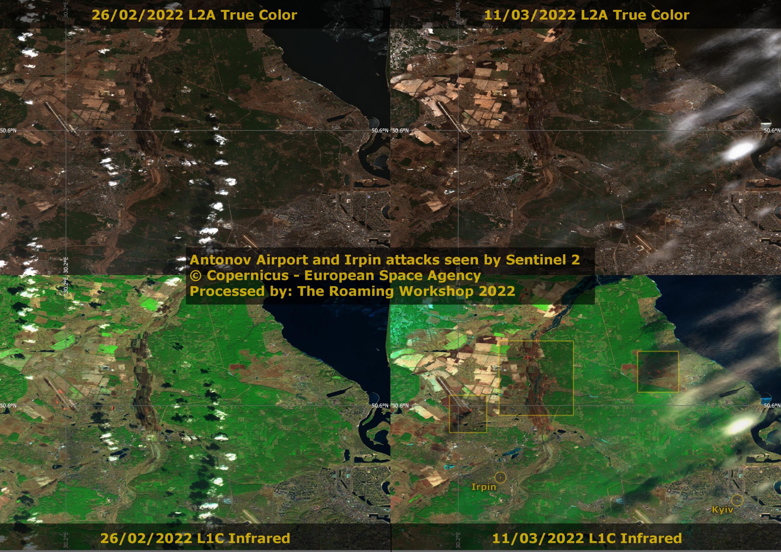
First Russian targets were aerodromes so air combat was neutralized. Antonov International Airport involved a tough battle from day 1
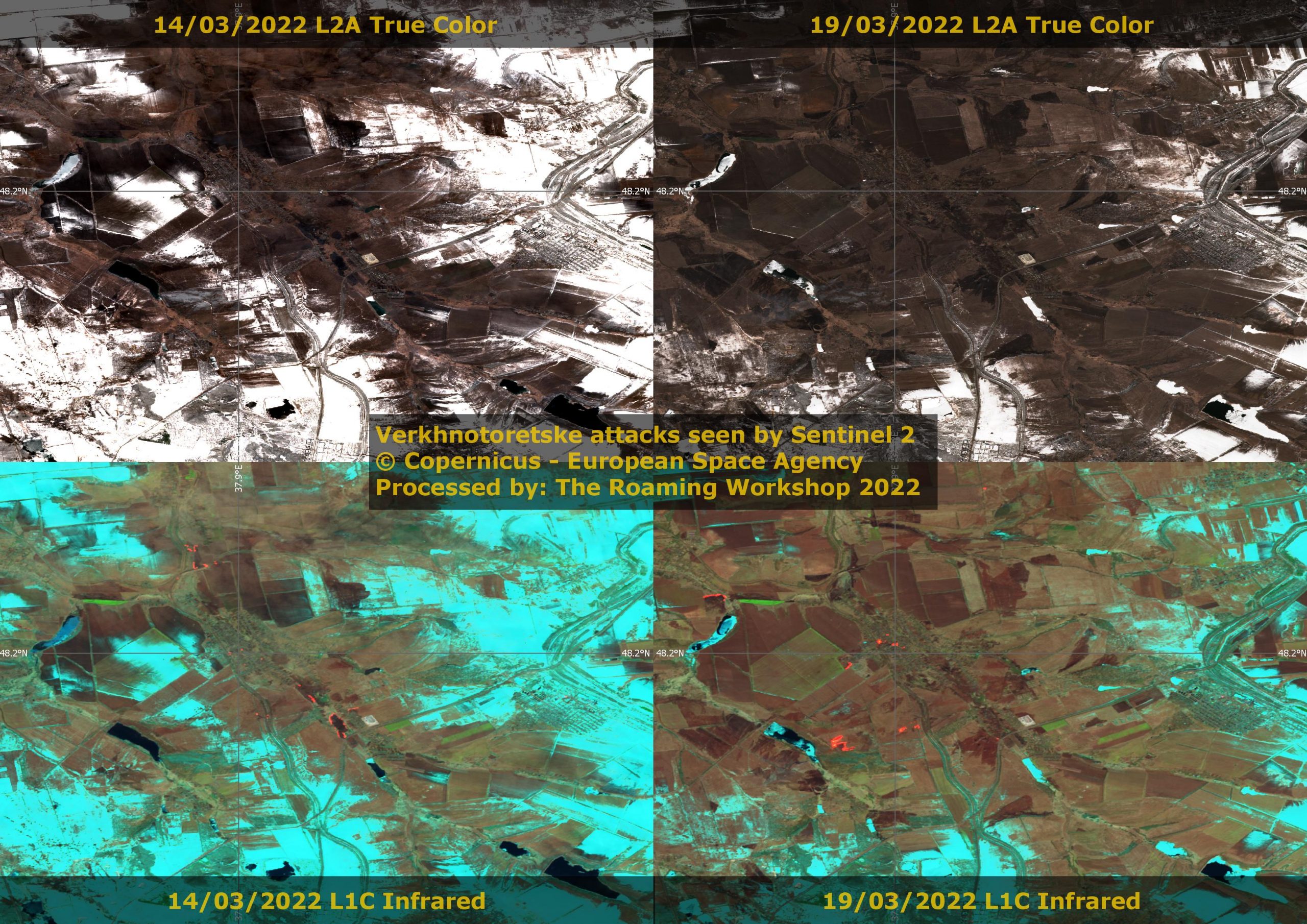
Verkhnotoretske village was an intense front for the first month, hardly 20km away from Donetsk
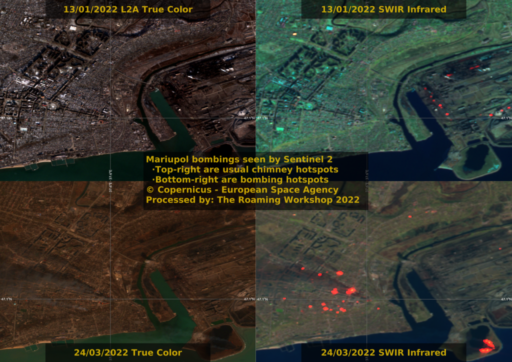
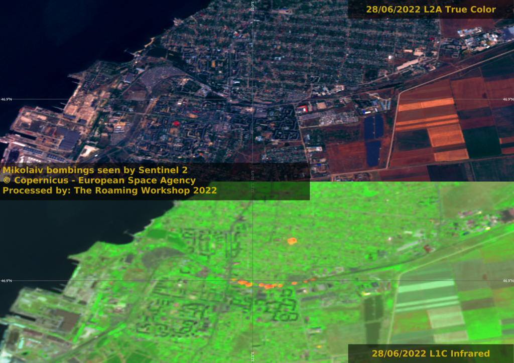
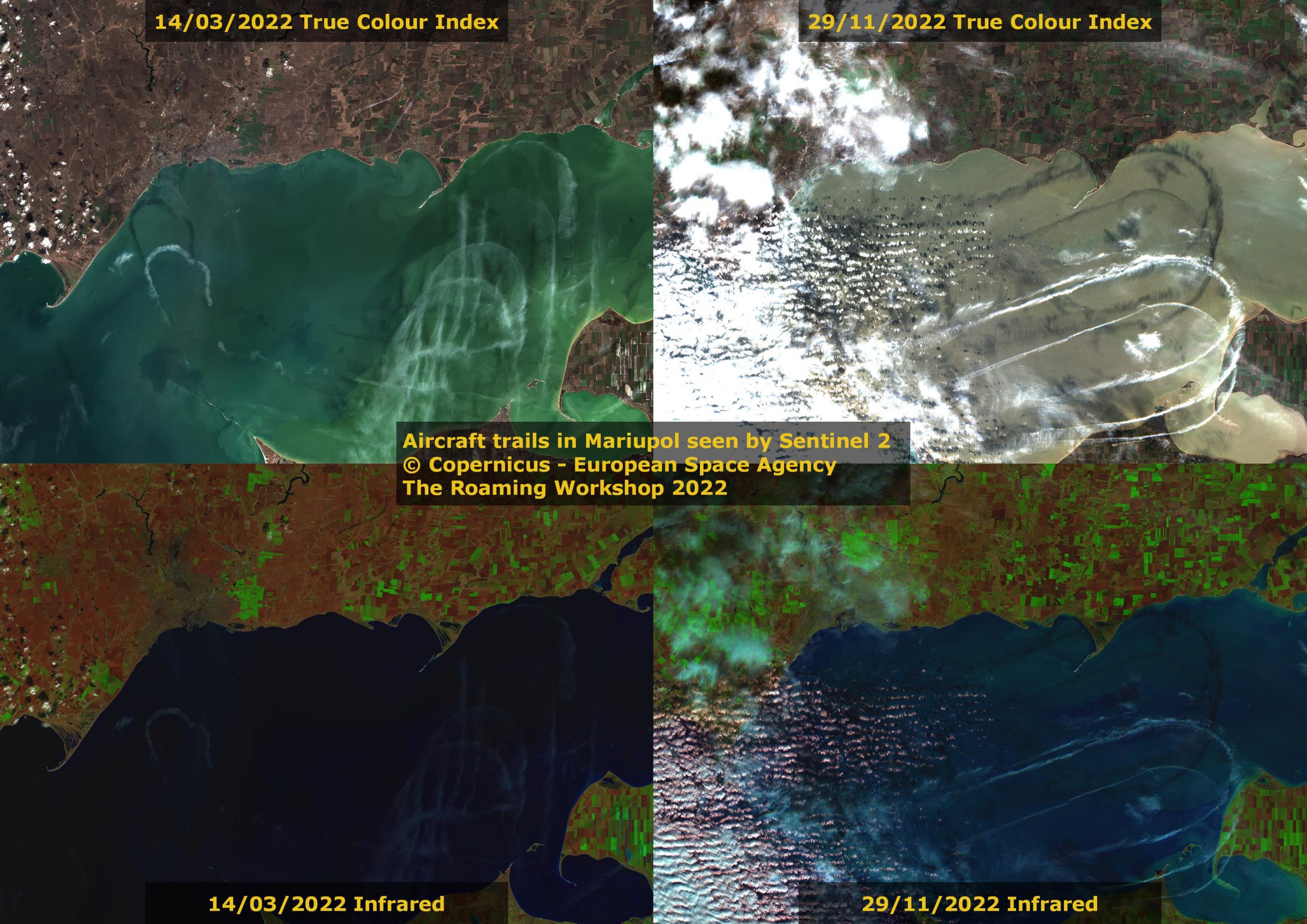
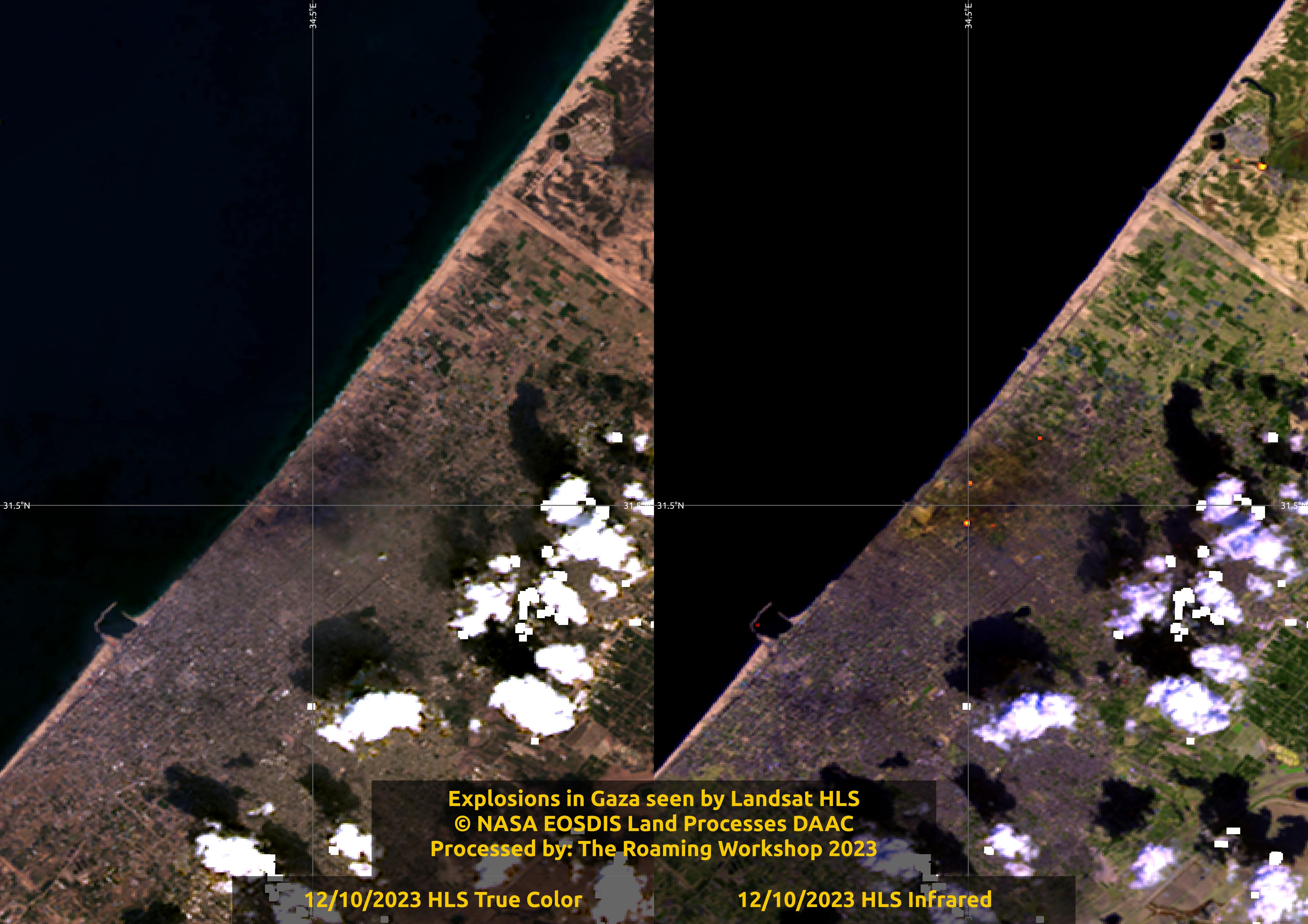
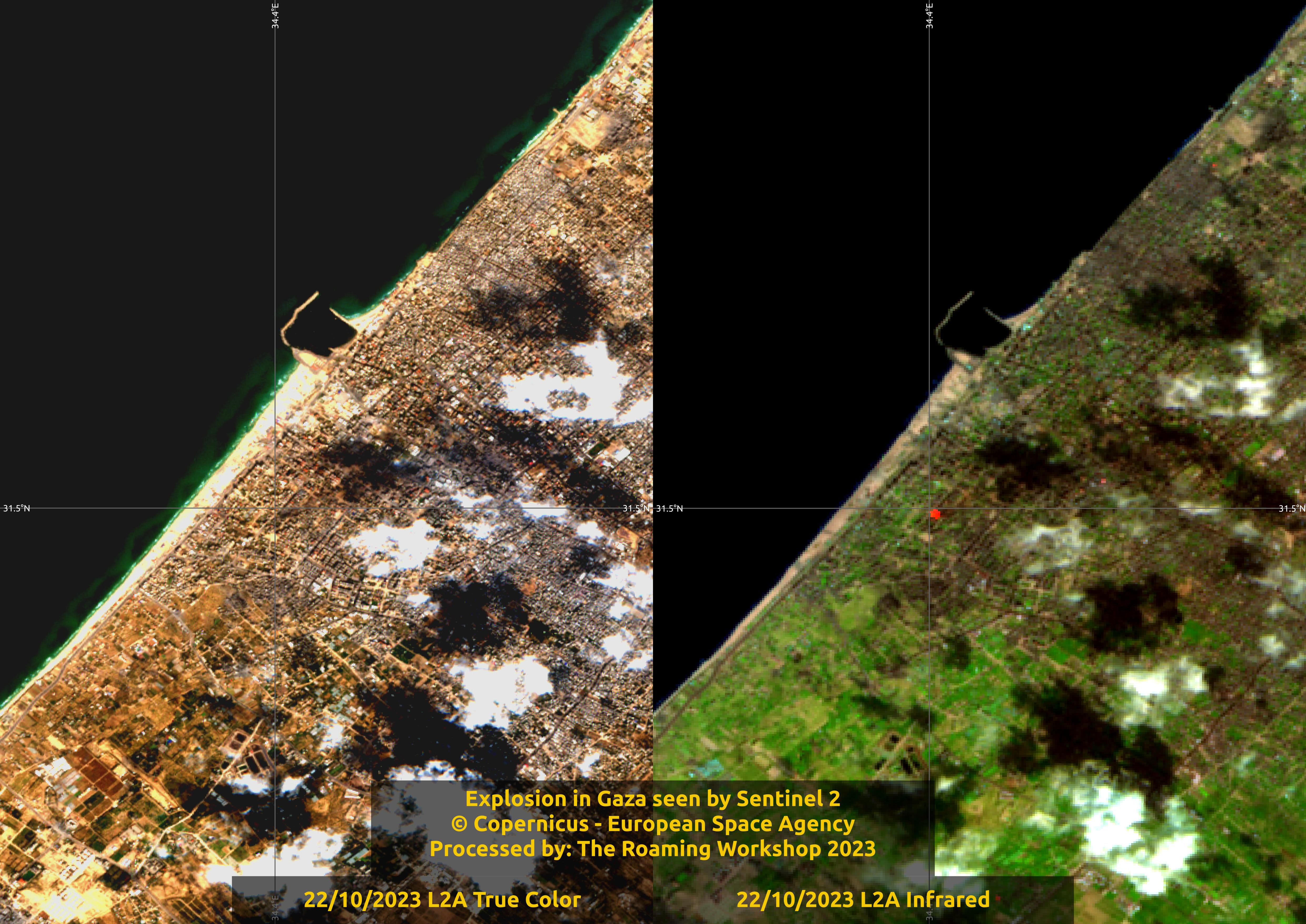
Mariupol was badly bombed at the start of the conflict. See the difference of usual infrared signal versus fires caused by bombs.
Mikolaiv's government building was half destroyed and 38 people died on 29th March.
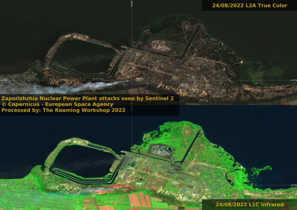
South of Zaporizhzhia is the biggest nuclear power plant in Europe. It was early attacked and occupied in March. Further combats, like this one in August, could cause a nuclear catasthrope.
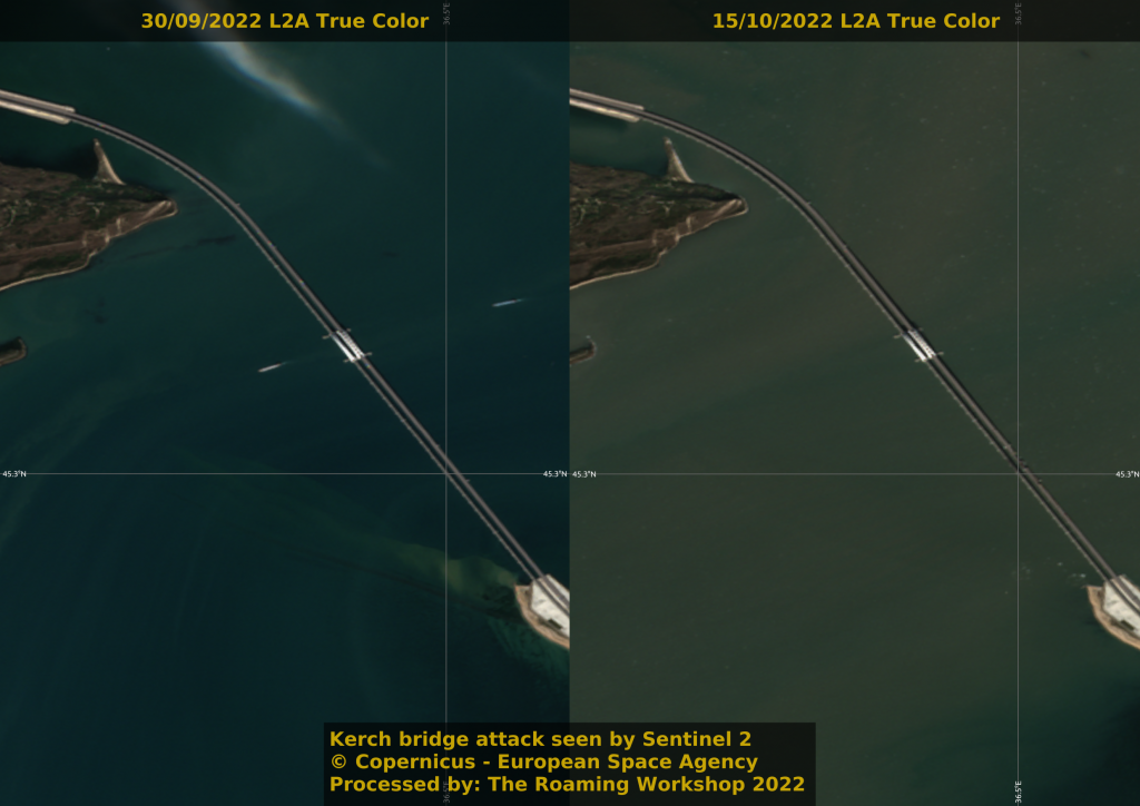
Claimed Crimea is connected to continental Russia via the Kerch bridge. A bomb-truck caused it's partial destruction in October 2022.
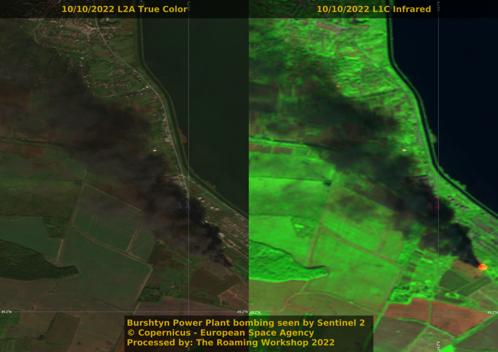
The attack in Kerch bridge led to a change in strategy and critical infrastructure for electricity and water have been targeted in sight of the coming winter.
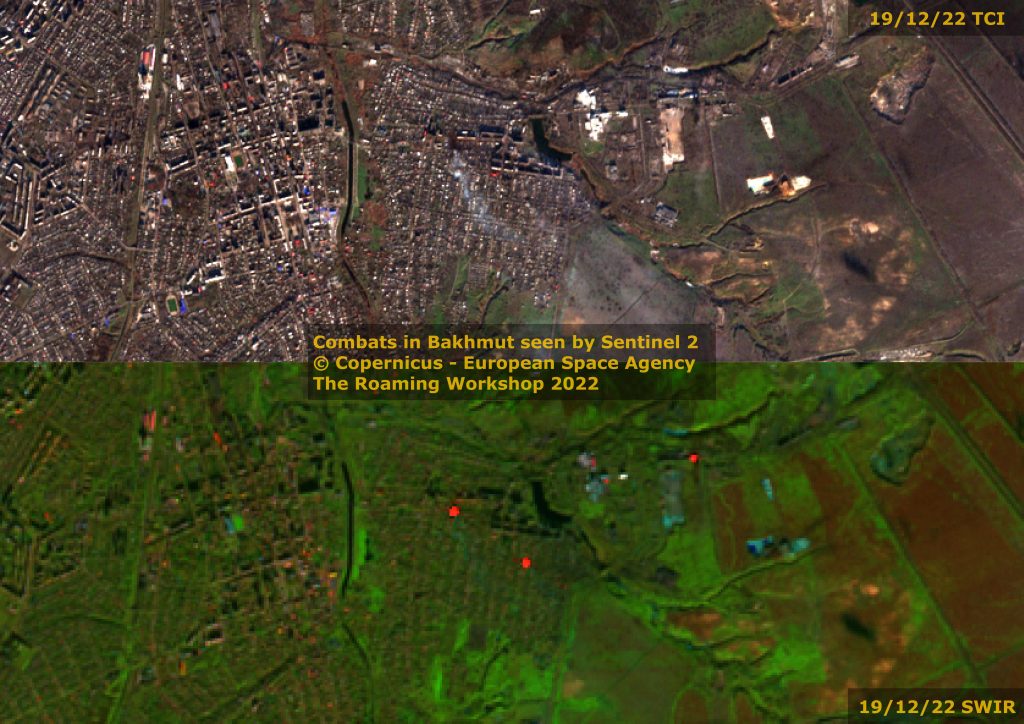
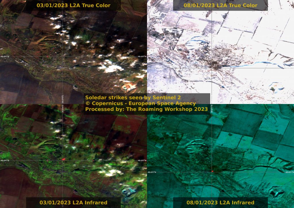
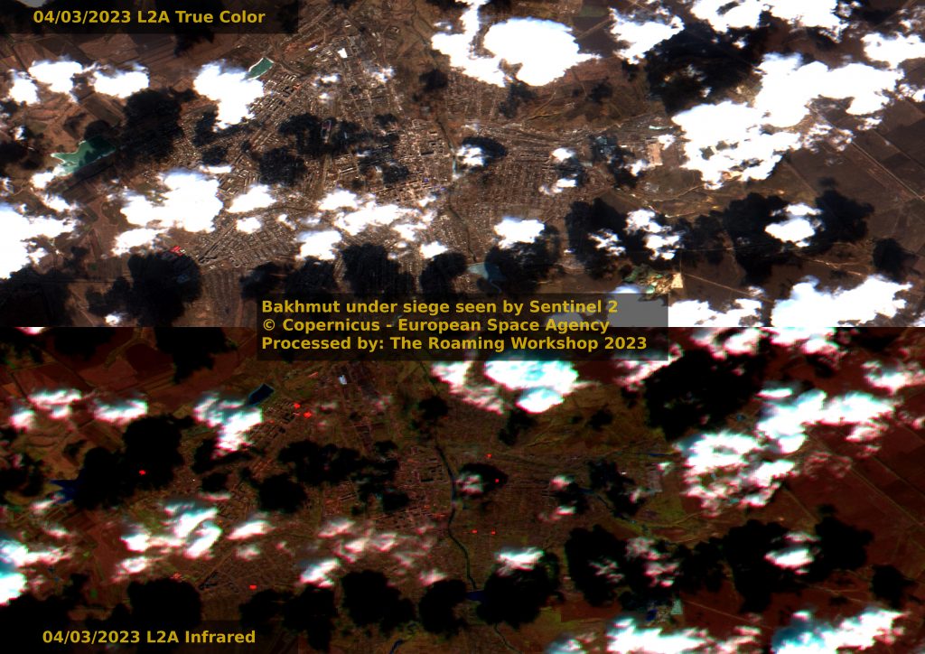
It's usually cloudy in Ukraine, but these clouds aren't usual. The trails left behind aircrafts are also seen from space, providing information on their routes and height. Residential streets in Bakhmut, key location for Donbas' offensive, are resulting the scene of fierce combats. Europe's biggest salt mine, in Soledar, consists of 200km of 30m high tunnels, useful to house troops and war equipment during winter, hardly 15km away from Bakhmut.
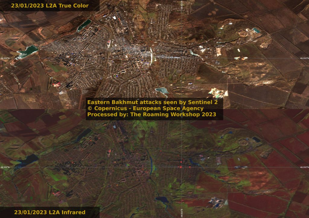
One month since I first spotted the battle for Bakhmut on a residential neighbourhood to the East.
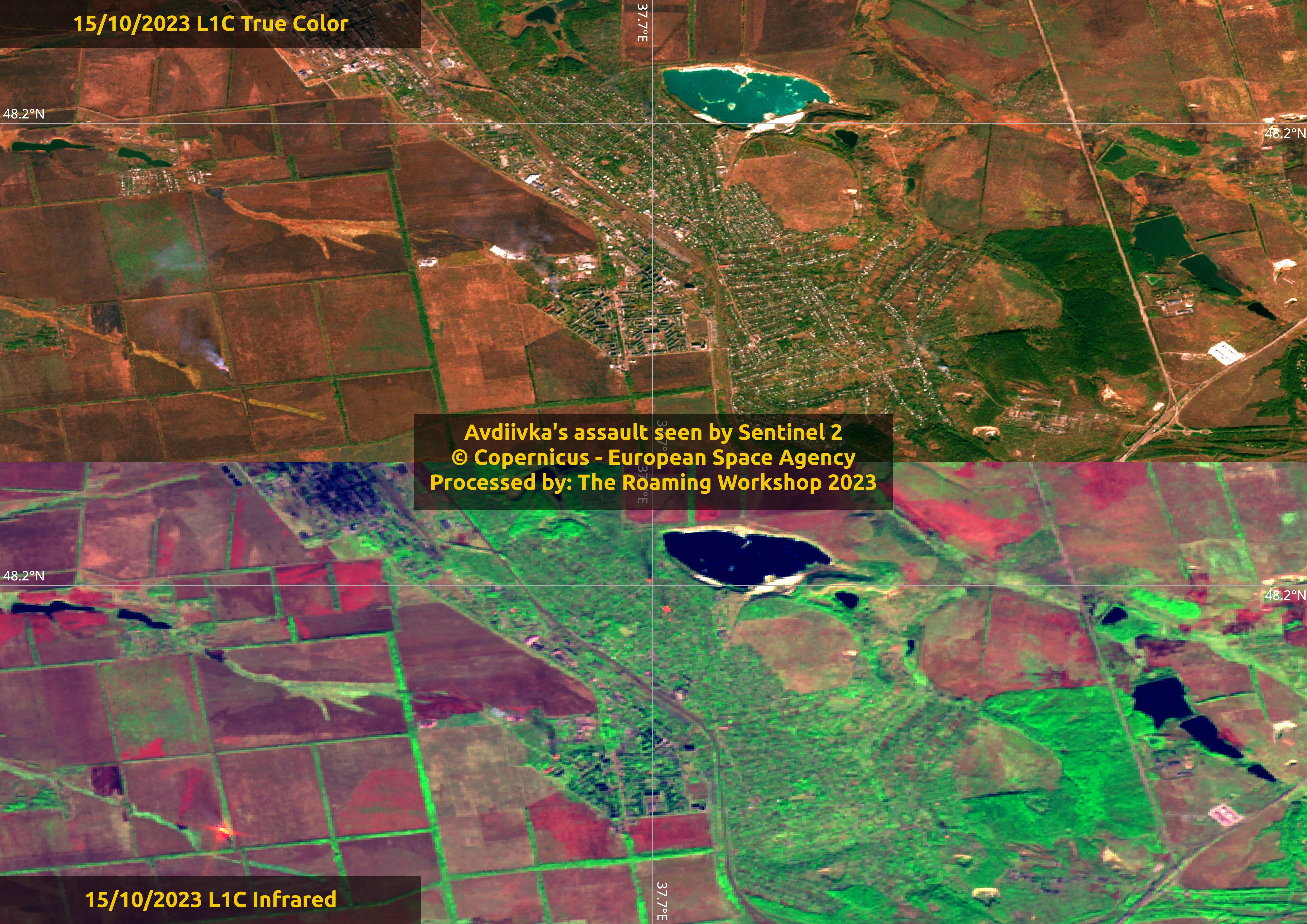
Infrared activity in Bakhmut doesn't cease being the hardest front of the war so far From 10th October 2023, the brutal attempts to capture Adviidka continues to cause deaths.
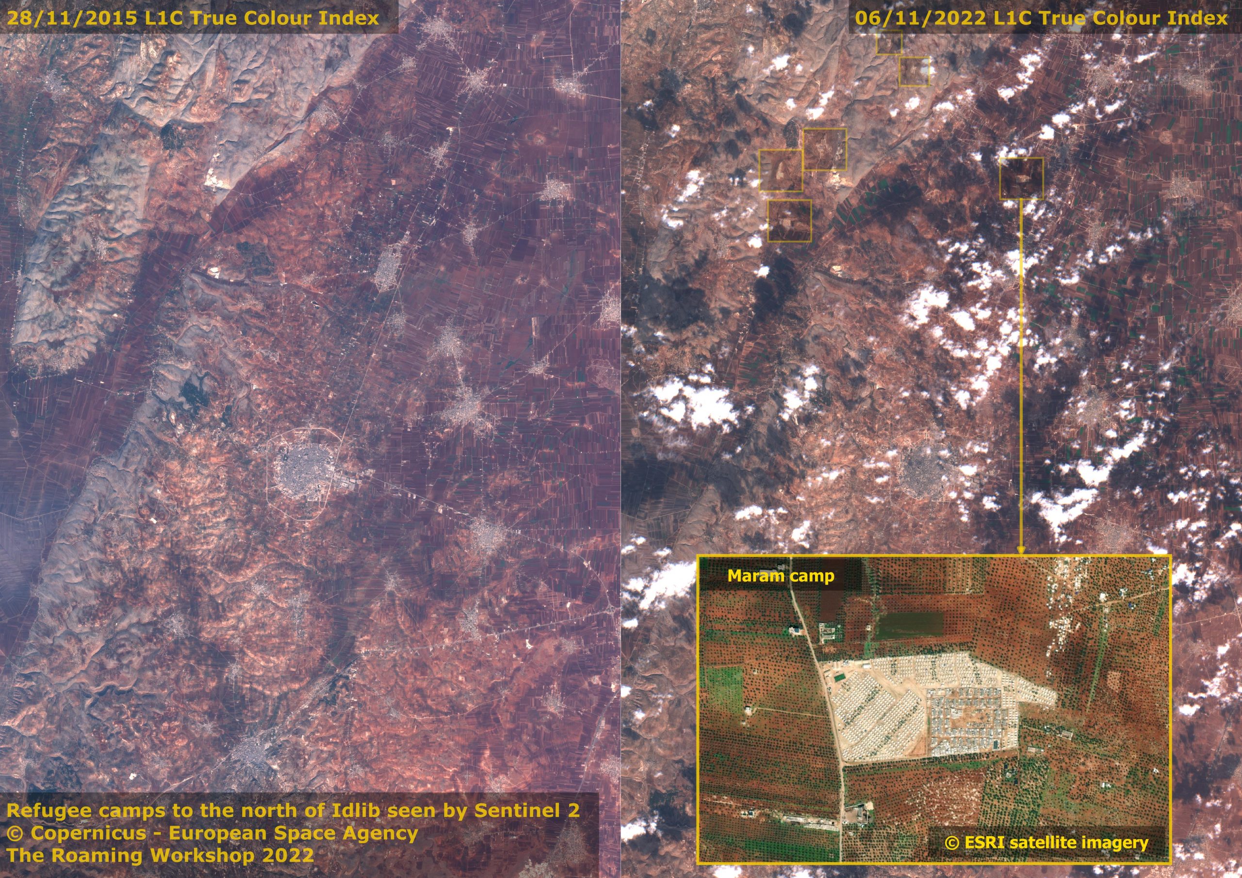
On November 6th 2022, attacks over refugee camps ended in 9 people killed (3 of them children). People has been displaced from their homes after destroying most major settlements. You can see there were no camps in this area in 2015.
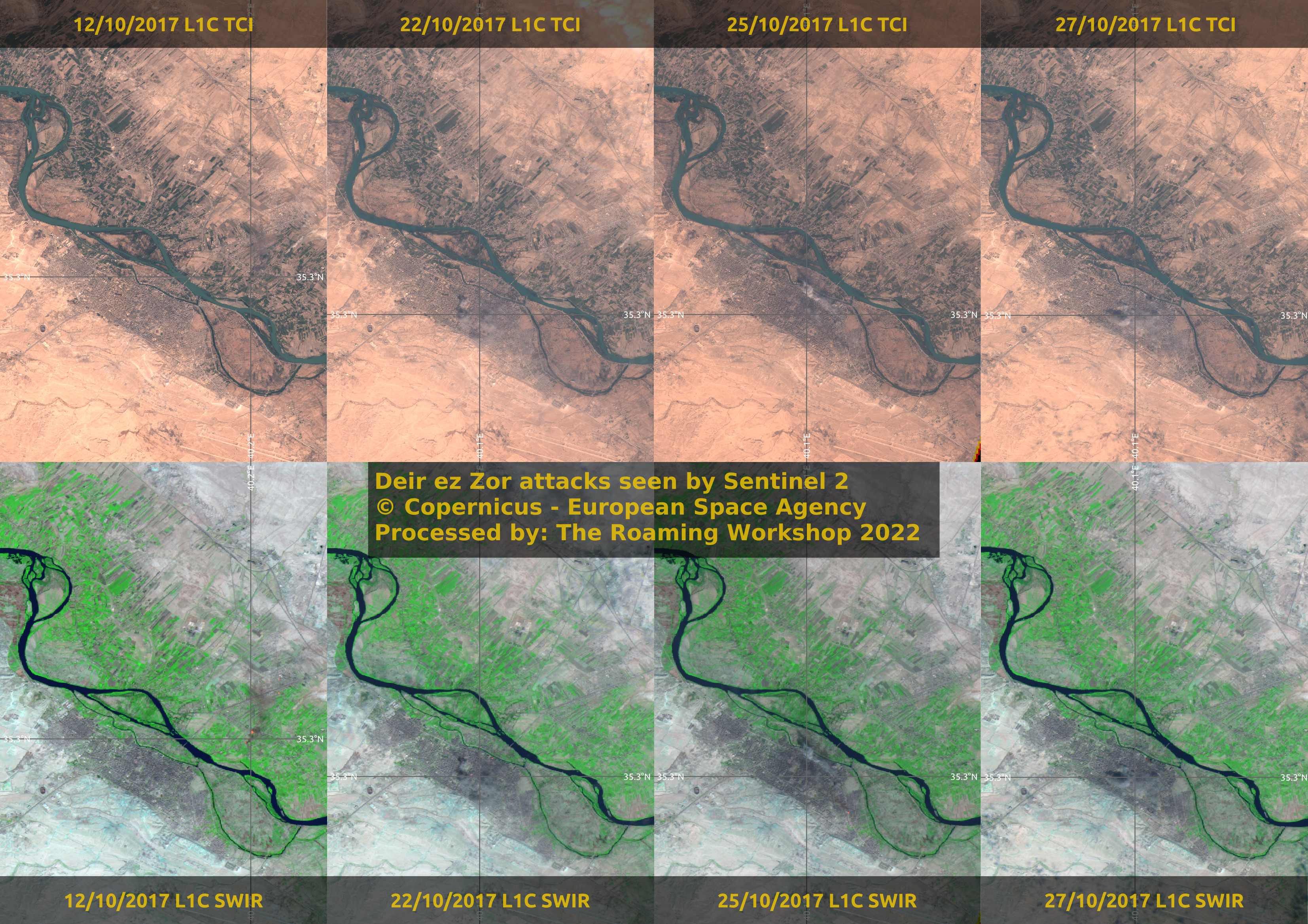
Late 2017 involved intense bombing of cities presumably occupied in northern and eastern Syria.
After a few posts about the use of satellite information, let’s see how to bring it (almost) all together in a practical and impacting example. And it’s given the latest wildfires occurred in Spain that they’ve called my attention as I could not imagine how brutal they have been (although nothing compared to the ones in Chile, Australia or USA). But let’s do the exercise without spending too much GB in geographical information.
What I want is to show the extent of the fire occurred in Asturias in March, but also to show the impact removing the trees affected by the flames. Let’s do it!
Content
Download data
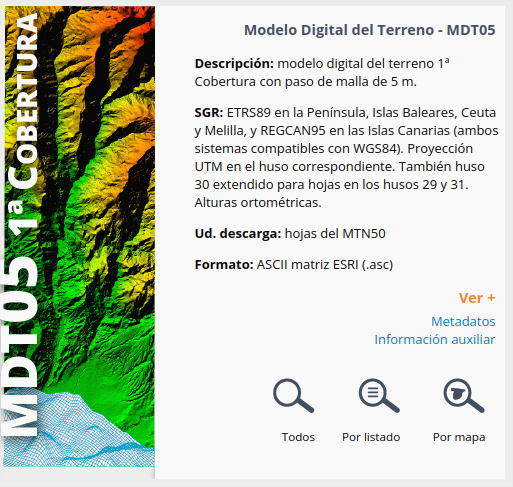
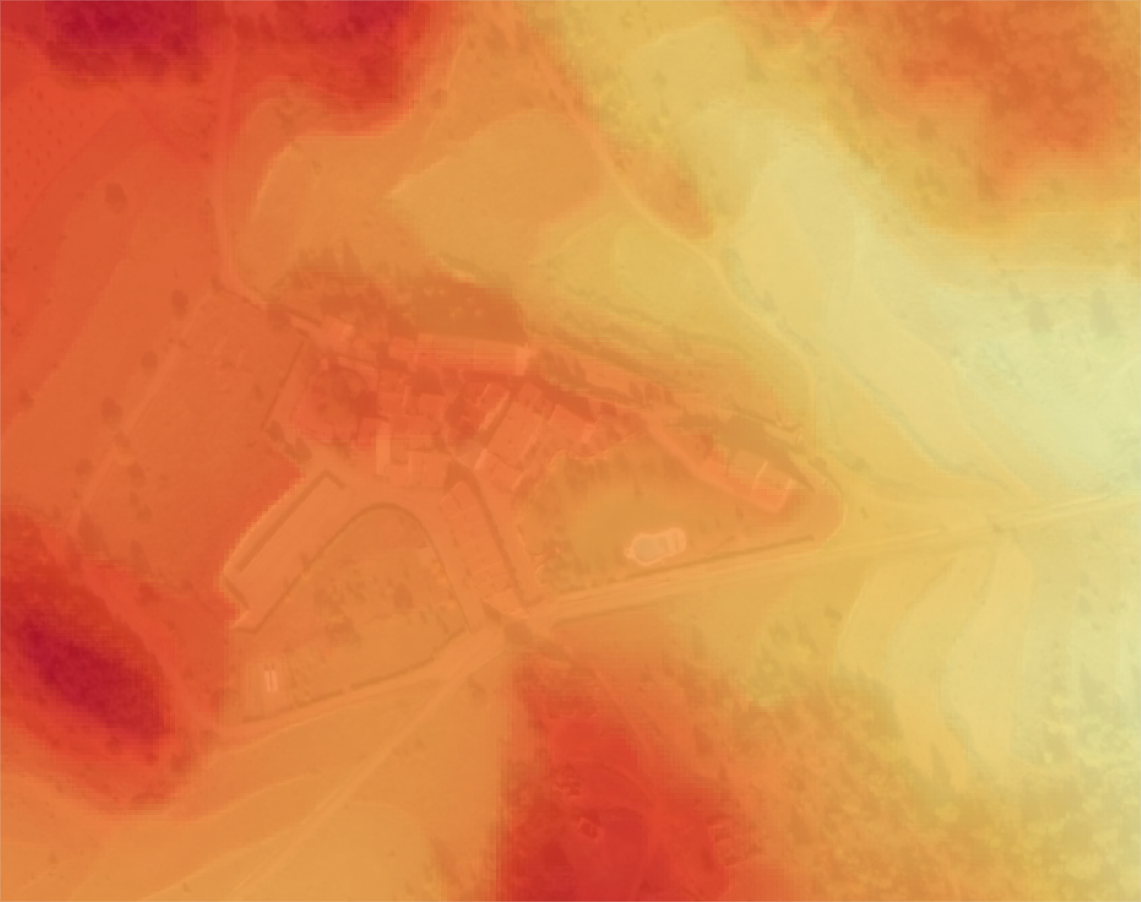
I will need a Digital Surface Model (which includes trees and structures), an orthophoto taken during the fire, and a Digital Terrain Model (which has been taken away trees and structures) to replace the areas affected by the fire.
1. Terrain models
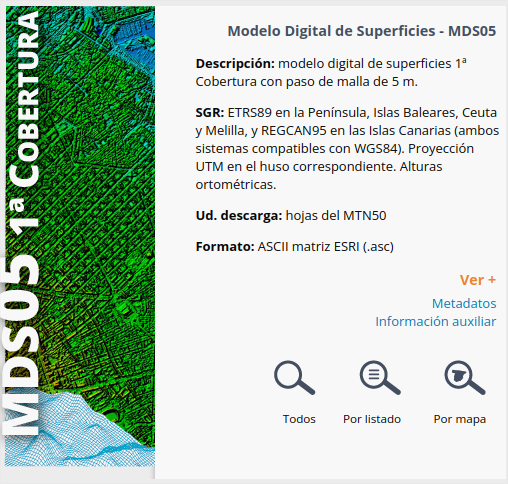
I'm going to use the great models from Spanish IGN, downloading the products MDS5 and MDT5 for the area.
We'll use the process i.group from GRASS in QGIS to group the different bands captured by the satellite in a single RGB raster, as we saw in this previous post:
You'll have to do it for every region downloaded, four in my case, that will be joint later using Build virtual raster
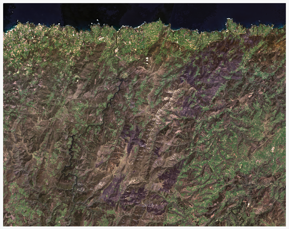
1. True color image (TCI)
Combine bands 4, 3, 2.
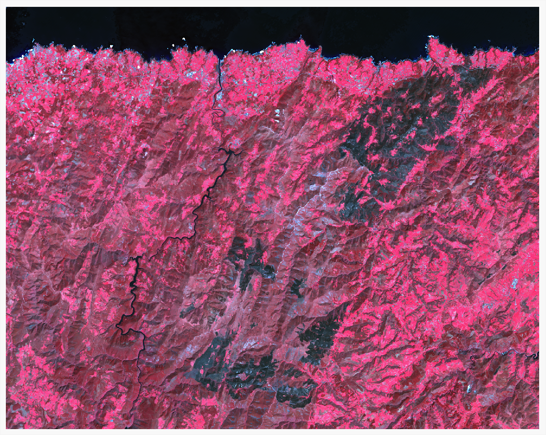
2. False color image
Combine bands 5, 4, 3.
3. Color adjustment
To get a better result, you can adjust the minimum and maximum values considered in each band composing the image. These values are found in the Histogram inside the layer properties.
here you have the values I used for the pictures above::
Band
TCI min
TCI max
FC min
FC max
1 Red
-100
1500
-50
4000
2 Green
0
1500
-100
2000
3 Blue
-10
1200
0
1200
Fire extent
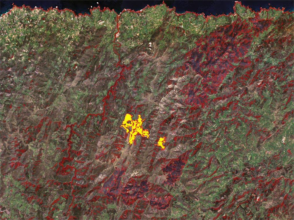
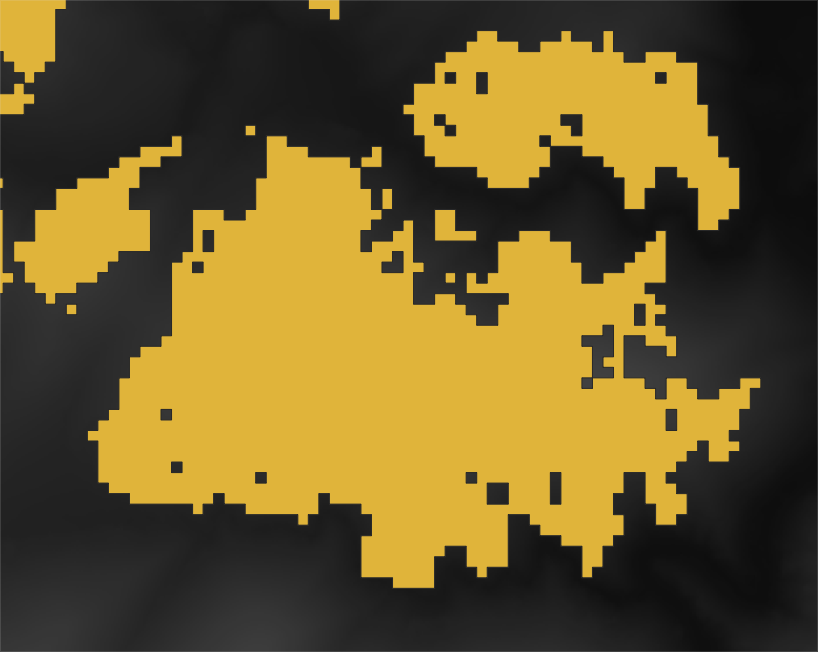
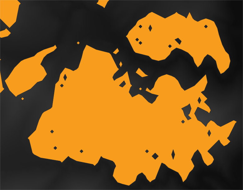
As you can see, the false color image shows a clear extension of the fire. We'll generate a polygon covering the extent of the fire with it.
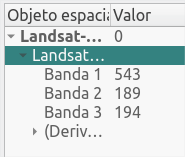
First, let's query the values in Band 1 (red) which offers a good contrast for values in the area of the fire. They are in the range 300-1300.
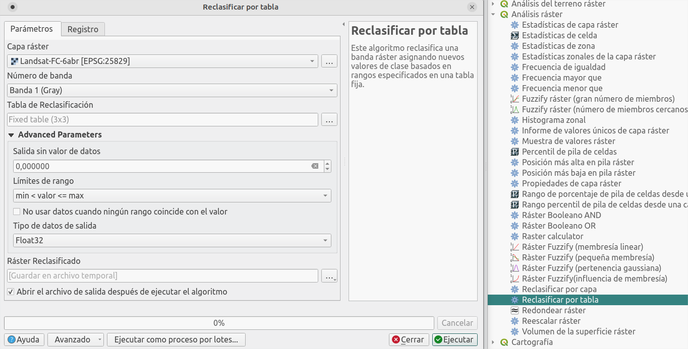
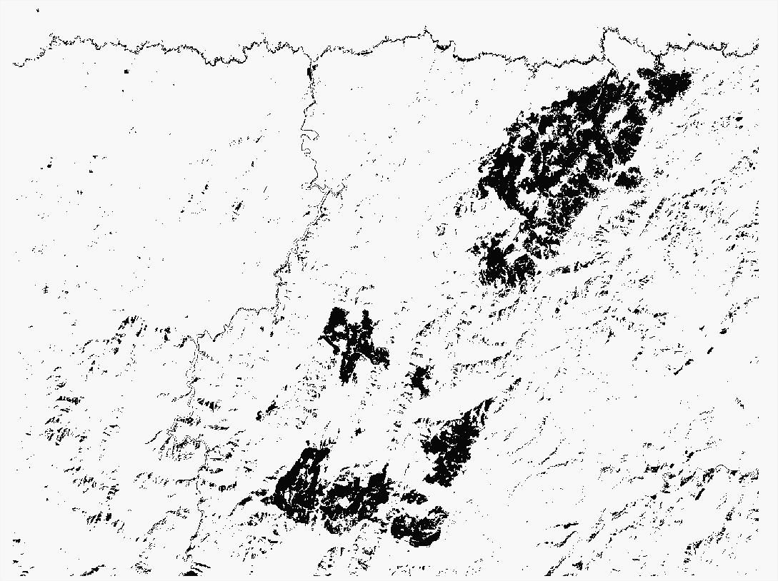
Using the process Reclassify by table, we'll assign value 1 to the cells inside this range, and value 0 to the rest.
Vectorize the result with process Poligonize and, following the satellite imagery, select those polygons in the fire area.
Use the tool Dissolve to merge all the polygons in one element; then Smooth to round the corners slightly.
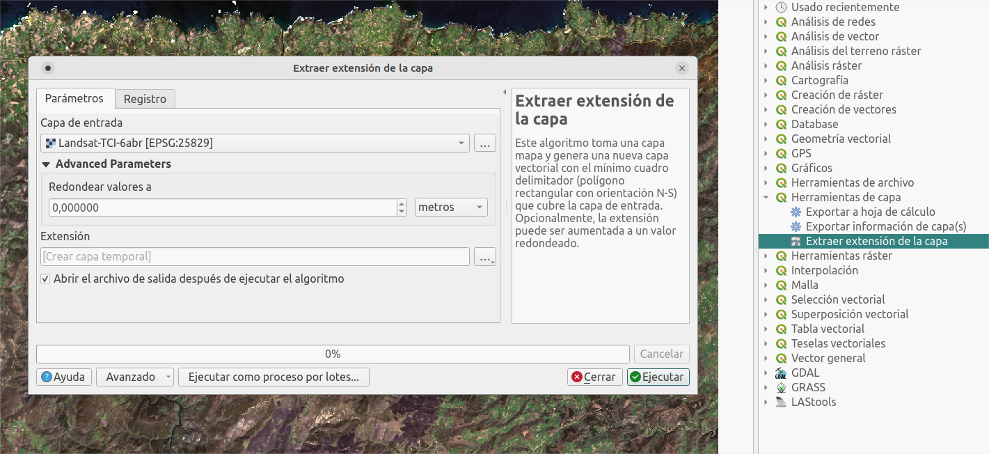
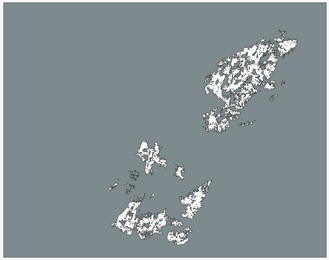
Let's now get the inverse. Extract by extent using the Landsat layer, then use Difference with the fire polygon.
Process terrain
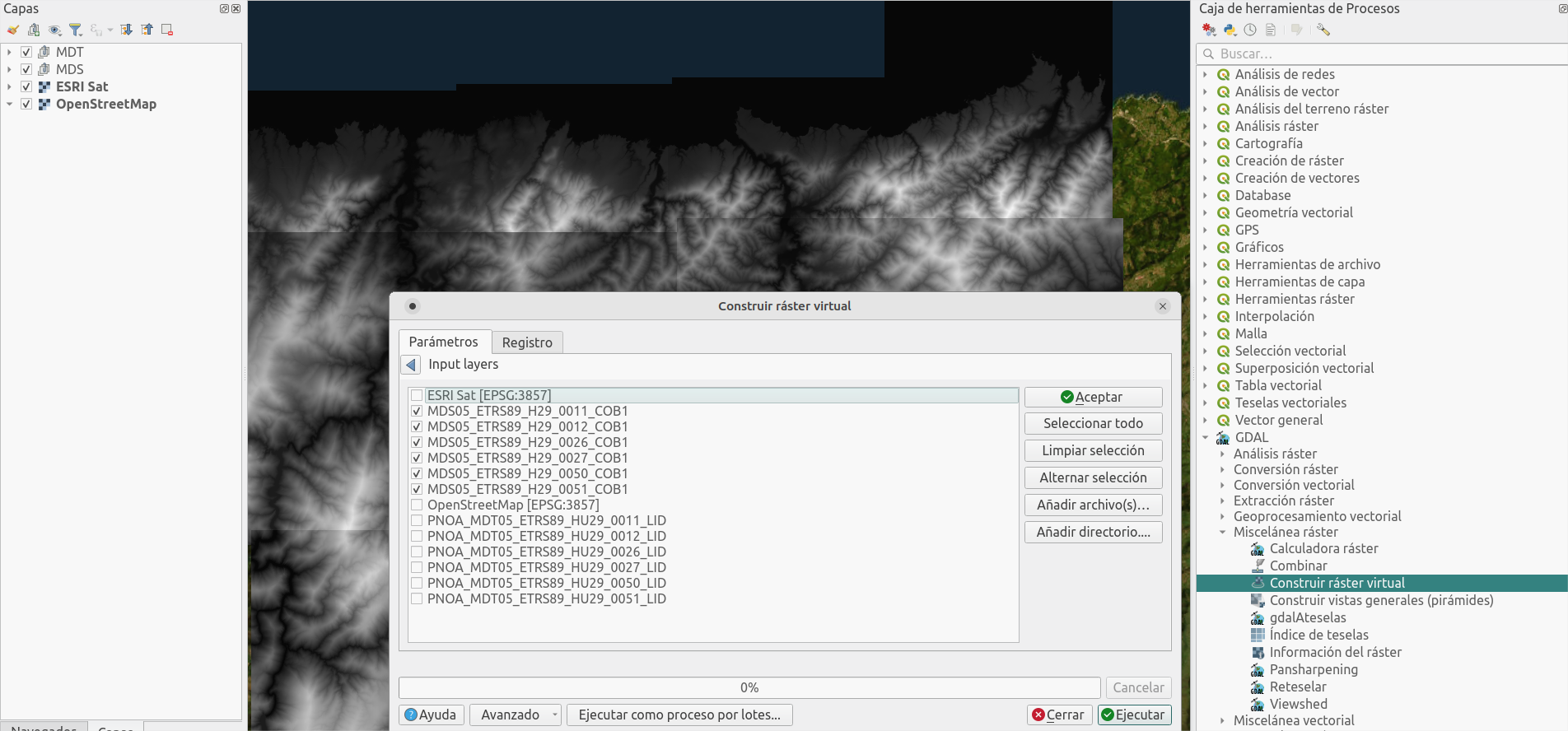
1. Combine terrain data
Join the same type model files in one (one for the DSM, and another one for the DTM). Use process Build virtual raster
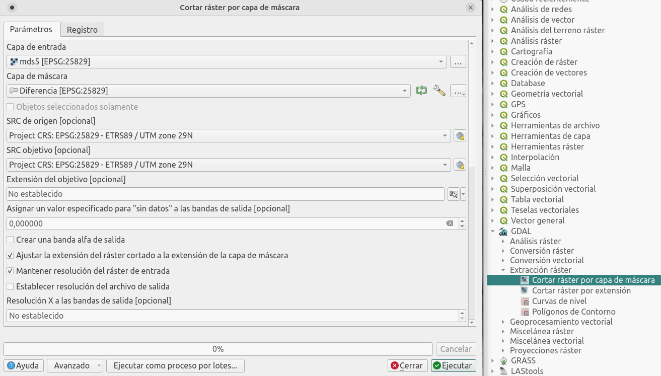
2. Extract terrain data
Extract the data of interest in each model:
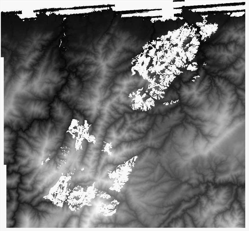
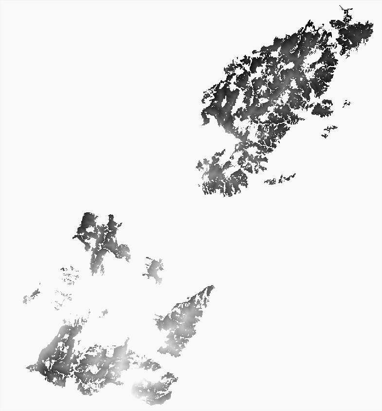
From the DSM extract the surface affected by the fire, so you'll remove all the surface in it.
Do the opposite with the DTM: keep the terrain (without trees) in the fire area, so it will fill the gaps in the other model.
Use the process Crop raster by mask layer using the layers generated previously.
Finally join both raster layers, so they fill each others' gaps, using Build virtual raster.
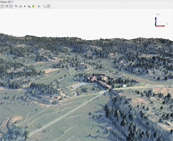
Bring it to life with Cesium JS
You should already have a surface model without trees in the fire area, but let's try to explore it in an interactive way.
I showed a similar example, using a custom Digital Terrain Model, as well as a recent satellite image, for the Tajogaite volcano in La Palma:
In this case I'll use Cesium JS again to interact easily with the map (follow the post linked above to see how to upload your custom files to the Cesium JS viewer).
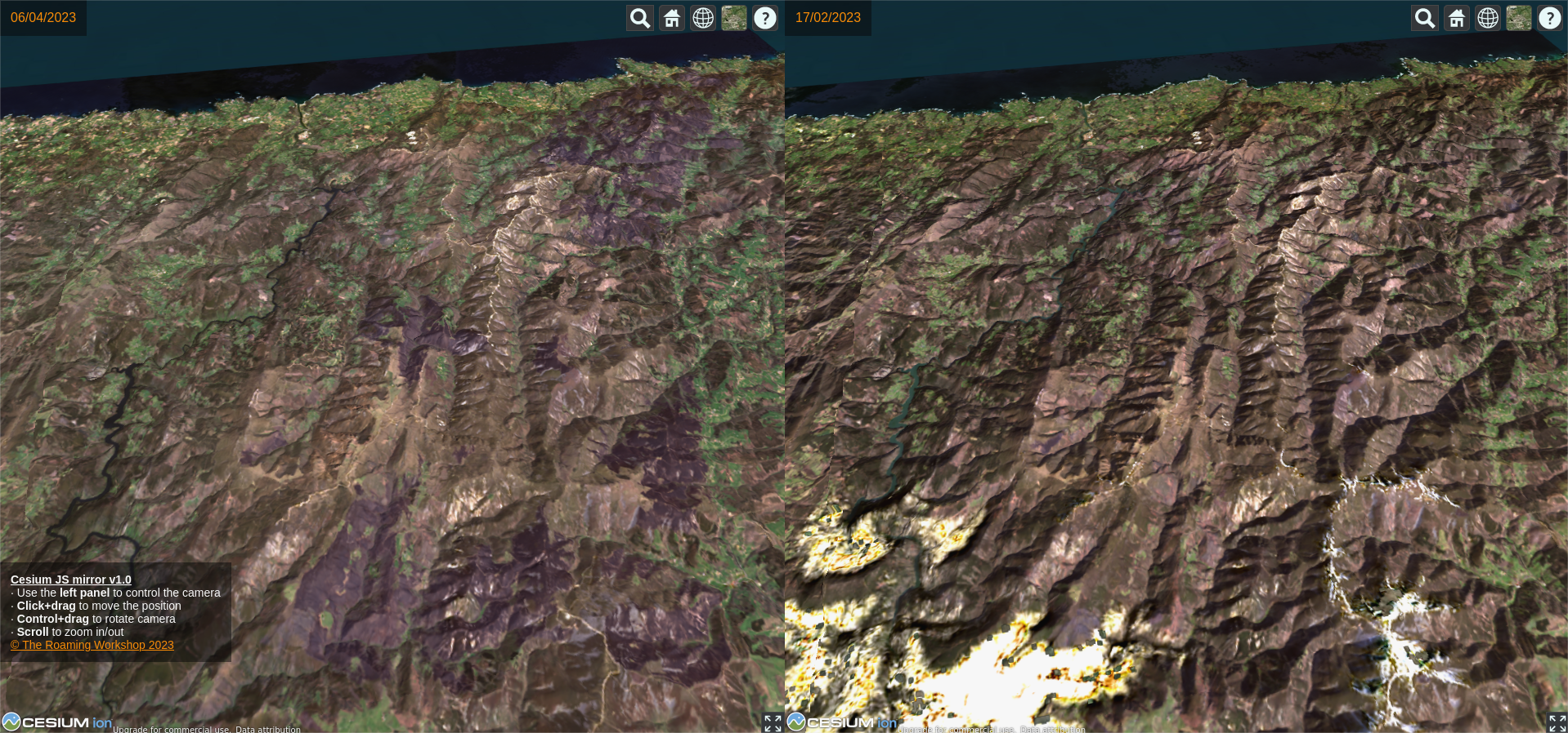
For this purpose, I created a split-screen viewer (using two separate instances of Cesium JS) to show the before and after picture of the fire. Here you have a preview:
I hope you liked it! here you have the full code and a link to github, where you can download it directly. And remember, share your doubts or comments on twitter!
Sometimes a Digital Terrain Model (DTM) might not be detailed enough or poorly cleaned. If you have access to LIDAR data, you can generate a terrain model yourself and make the most of the raw information giving more detail to areas of interest. Let’s see how.
Content
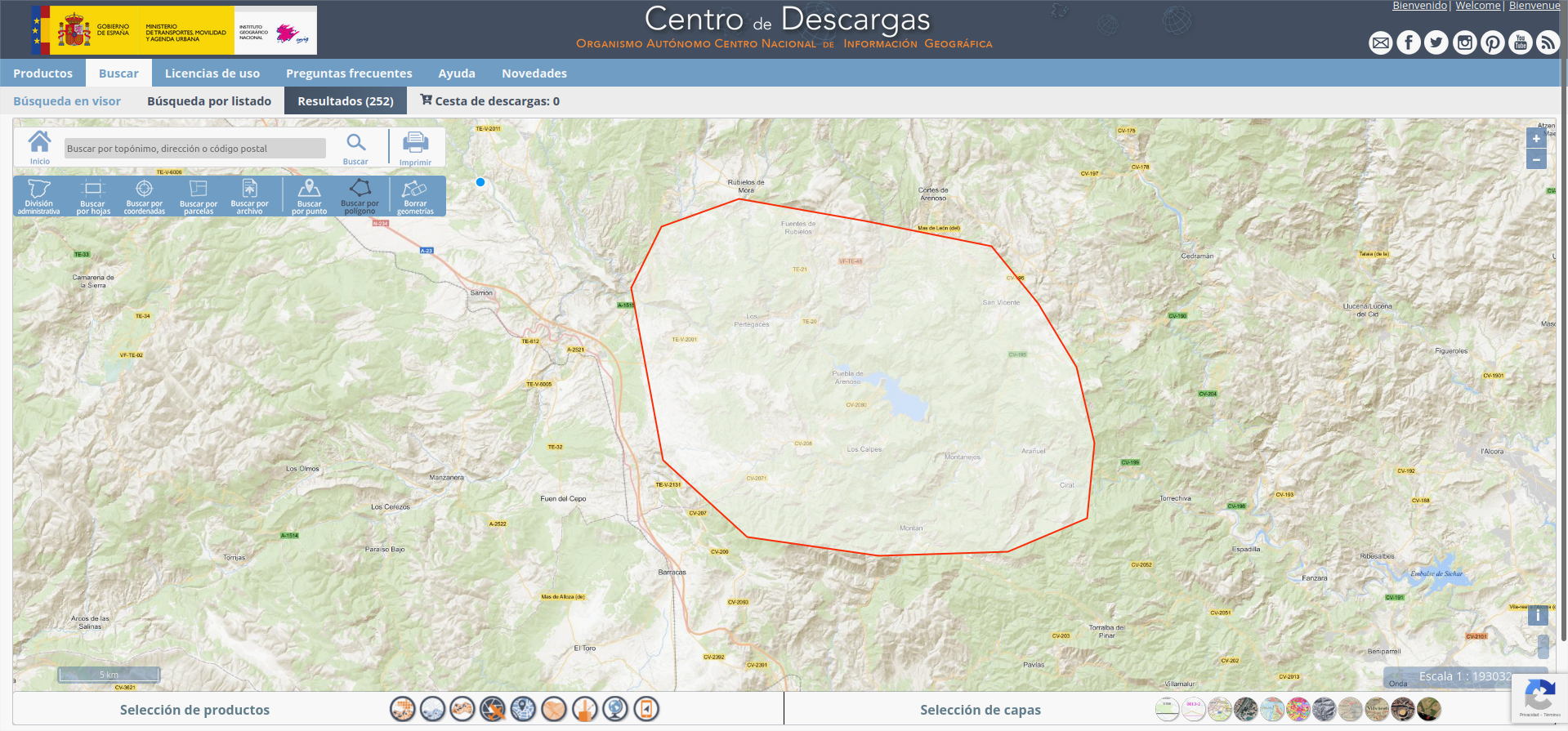
1. Data download
Point cloud
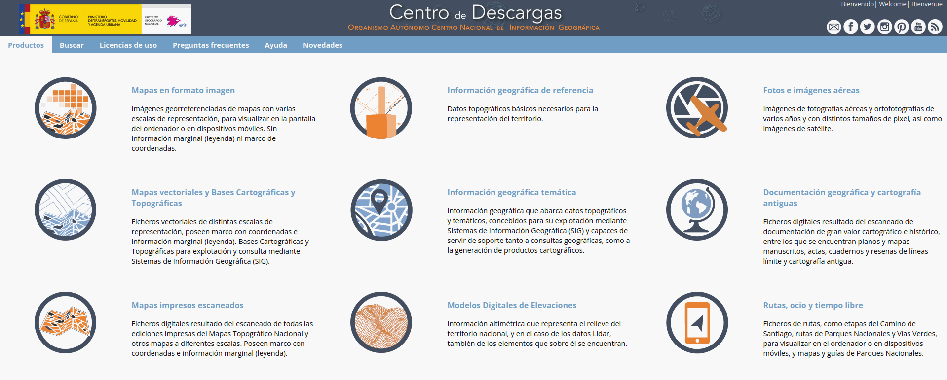
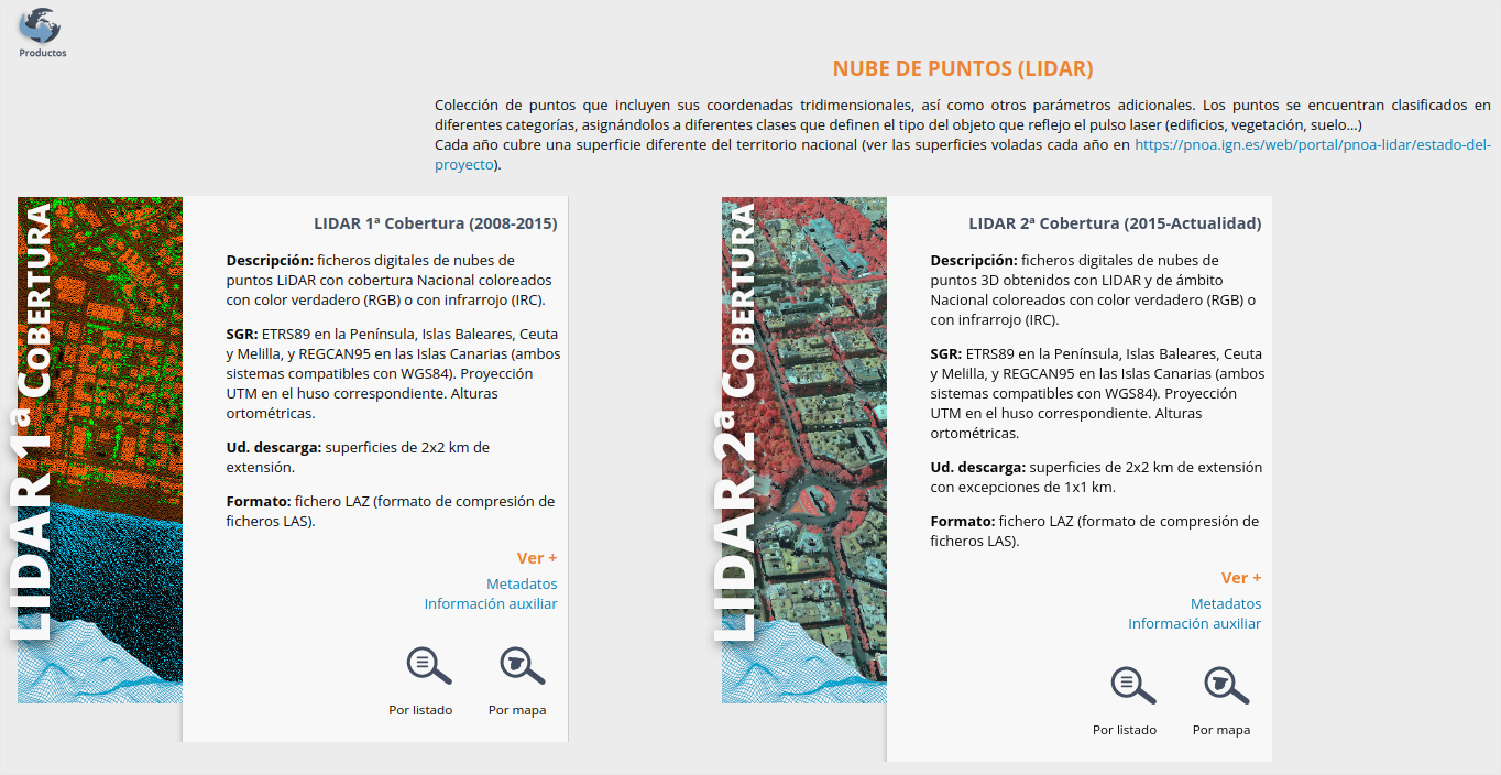
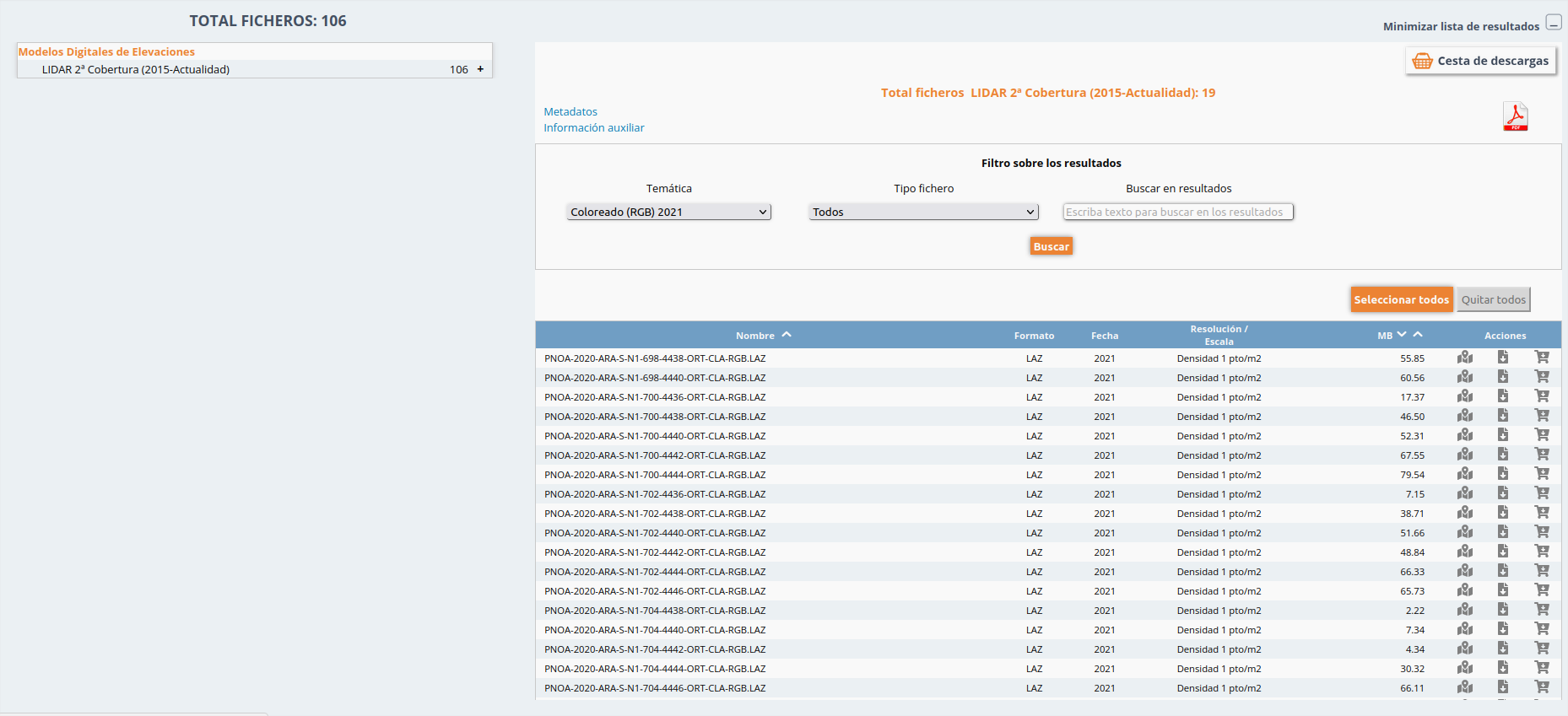
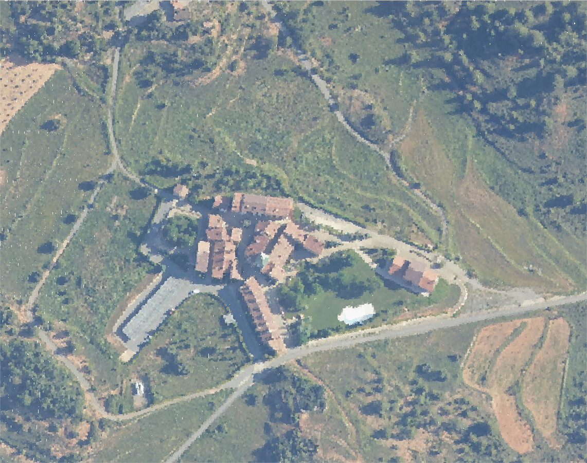
I'll use the awesome public data from the Spanish Geographical Institute (IGN) obtained with survey flights using laser measurements (LIDAR).
Download the files PNOA-XXXX...XXXX-RGB.LAZ. RGB uses true color; ICR, infra-red. But both are valid.
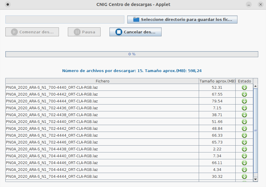
TIP! Download all files using the IGN applet. It's a .jnlp file that requires Java instaled on Windows or IcedTea on Linux (sudo apt-get install icedtea-netx)
2. Process LIDAR point cloud in QGIS
Direct visualization
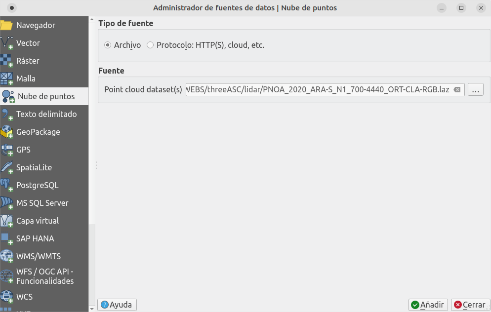
From the latest versions (like 3.28 LTR Firenze), QGIS includes compatibility with point cloud files.
Just drag and drop the file to the canvas or, in the menu, Layer -> Add layer... -> Add point cloud layer...
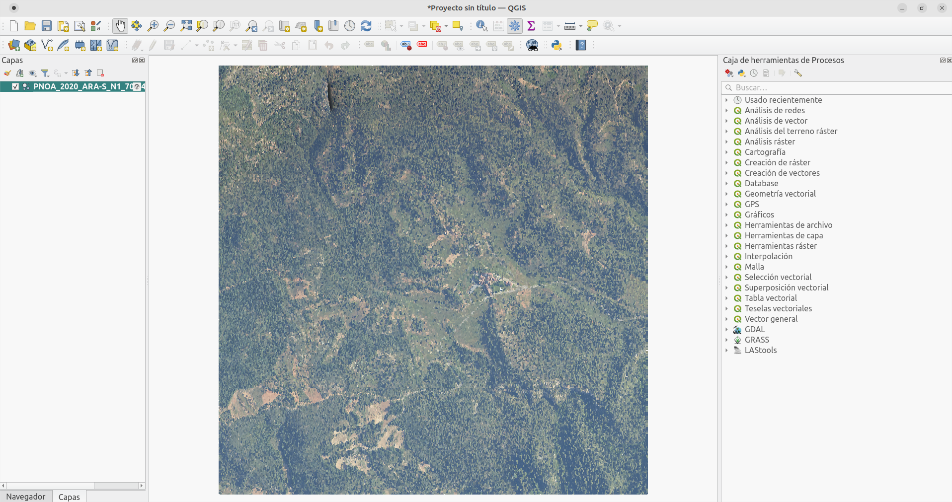
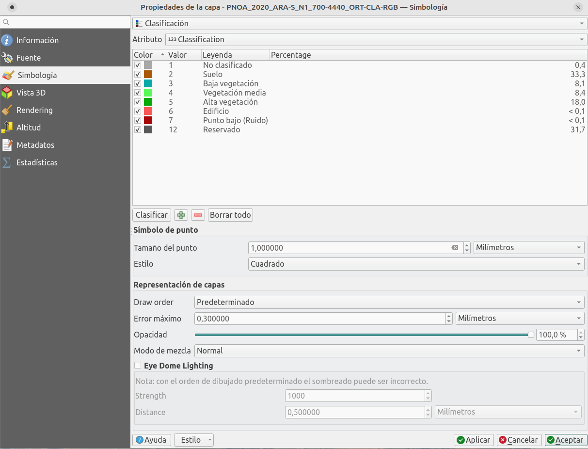
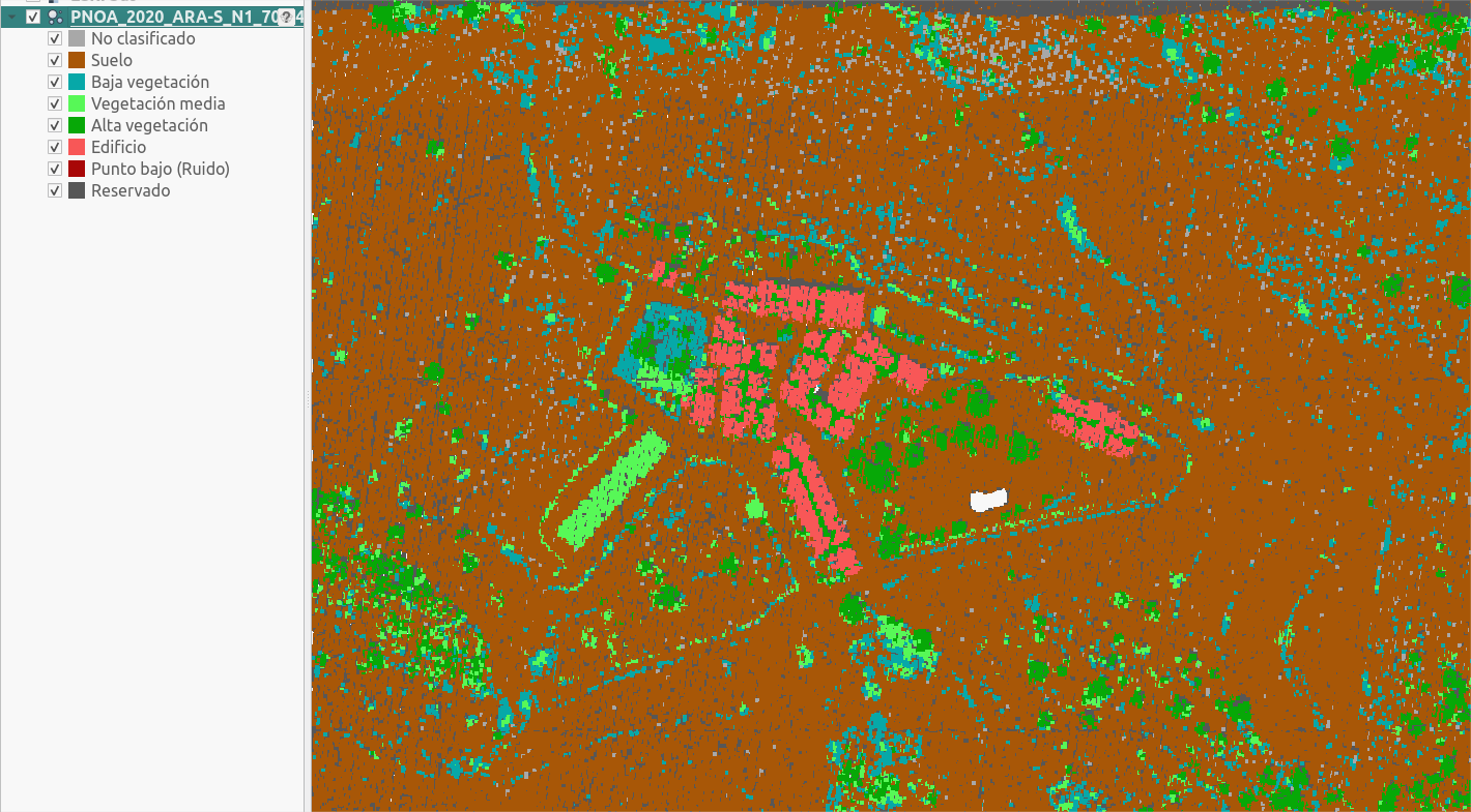
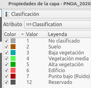
You'll see the true color data downloaded, which you can classify in the SimbologyProperties, choosing Clasification by data type:
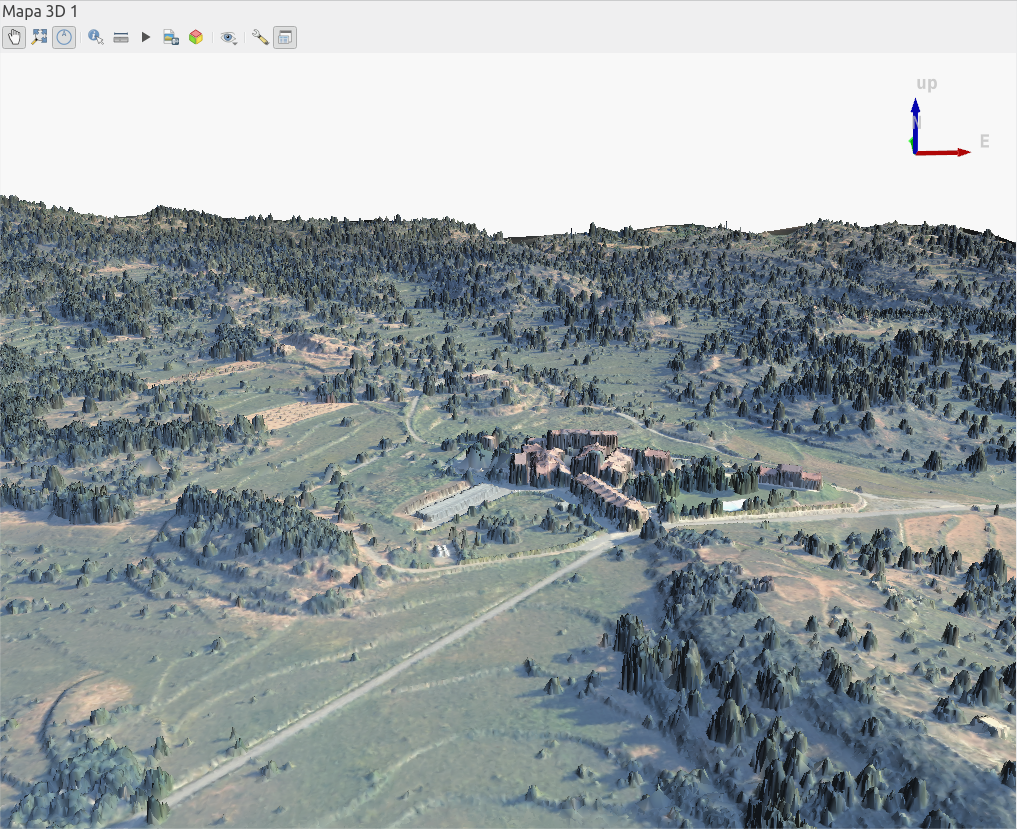
3D view
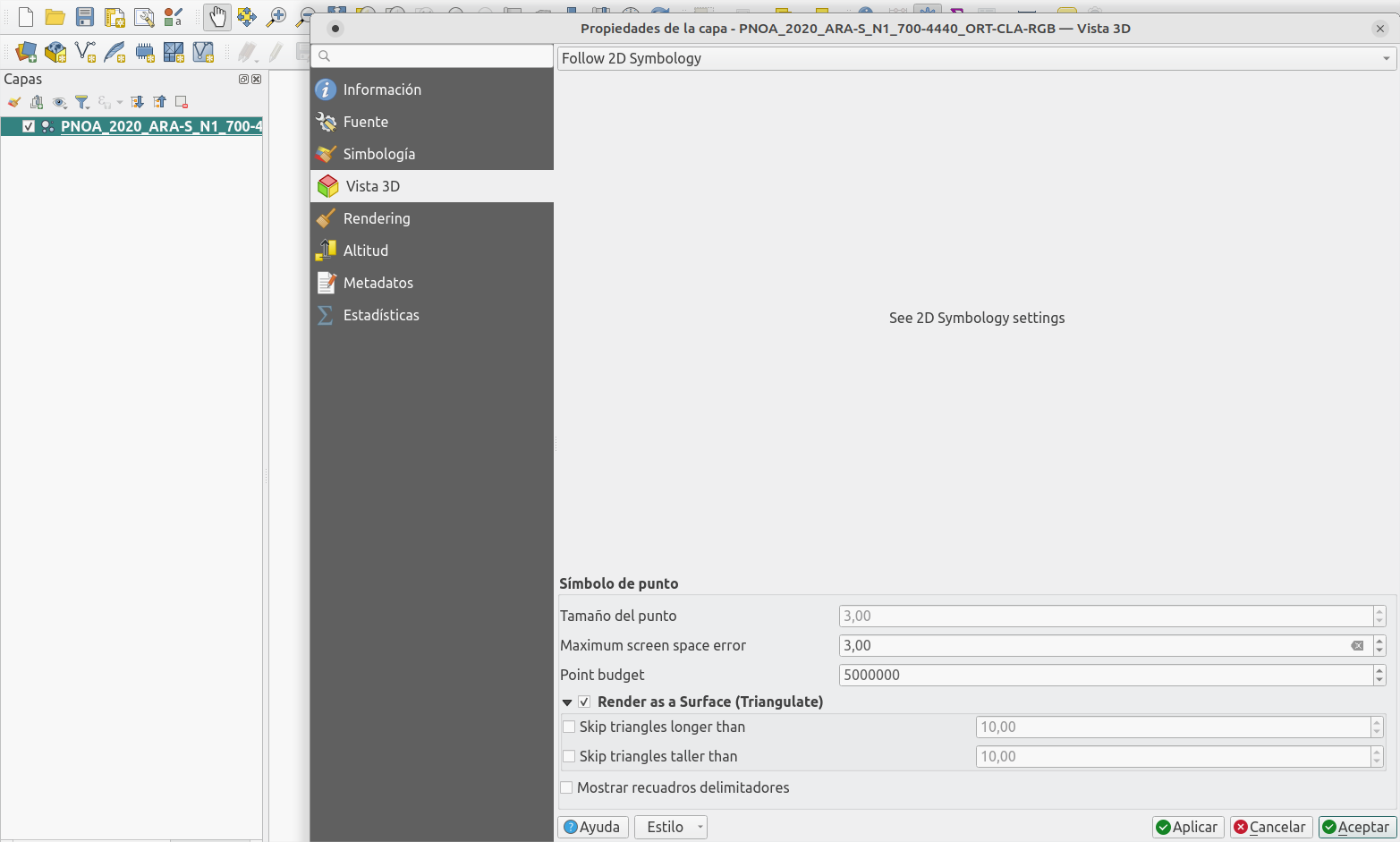
Another default function coming with QGIS is 3D visualization of the information.
Let's configure the 3D properties of the LIDAR layer to triangulate the surface and get a better result.
Now, create a new view in the menu View -> 3D Map Views -> New 3D map view. Using SHIFT+Drag you can rotate your perspective.
LAStools plugin
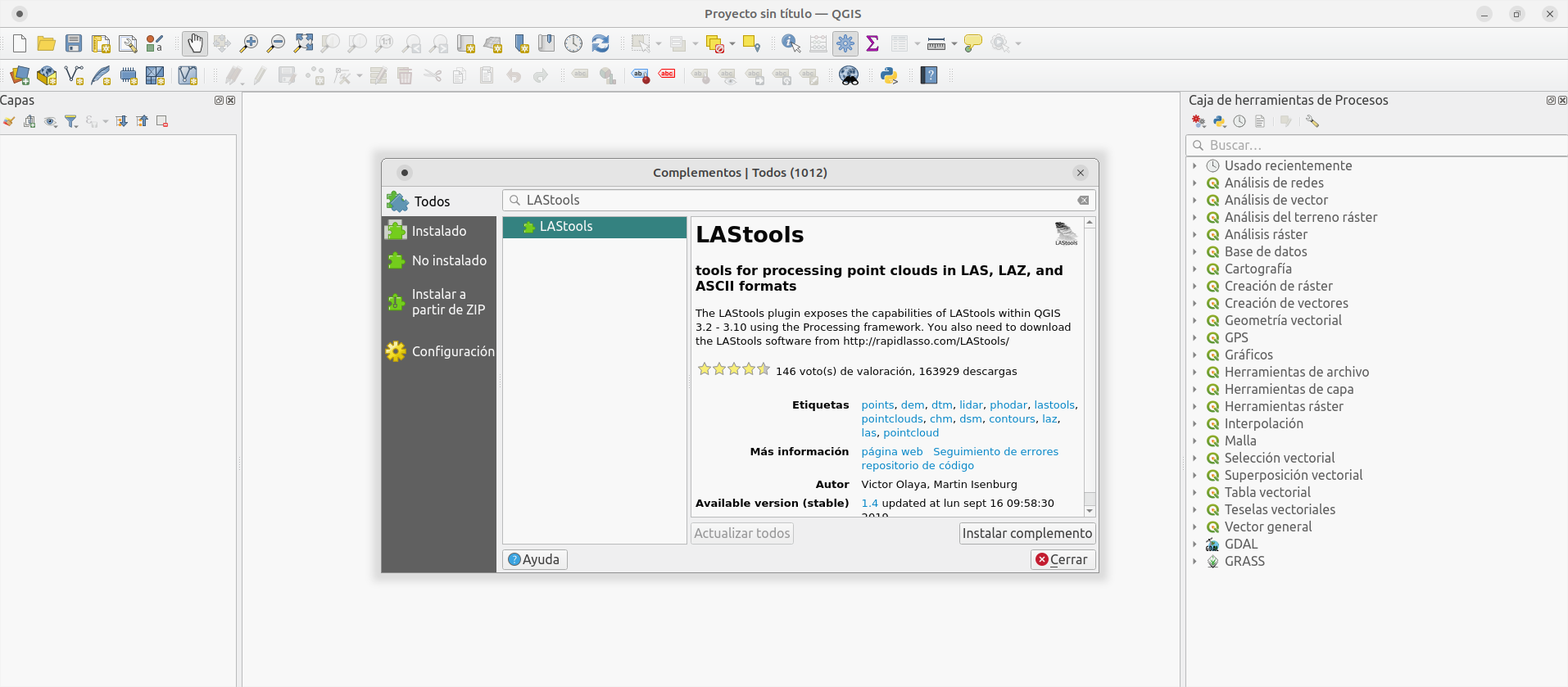
To handle LIDAR information easily we'll use the tools from a plugin called LAStools, which you can install in the following way:
TIP! On Linux it's recommended to install Wine to use the .exe files directly, or otherwise you'll need to compile the binaries.
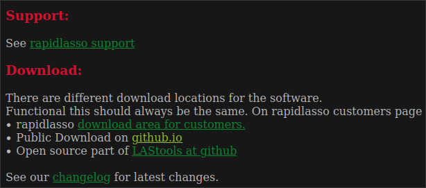
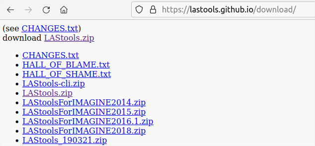
Access LAStools' website and scroll to the bottom:
The full tool comes to a price, but you can access the public download to use the basic functions that we need.
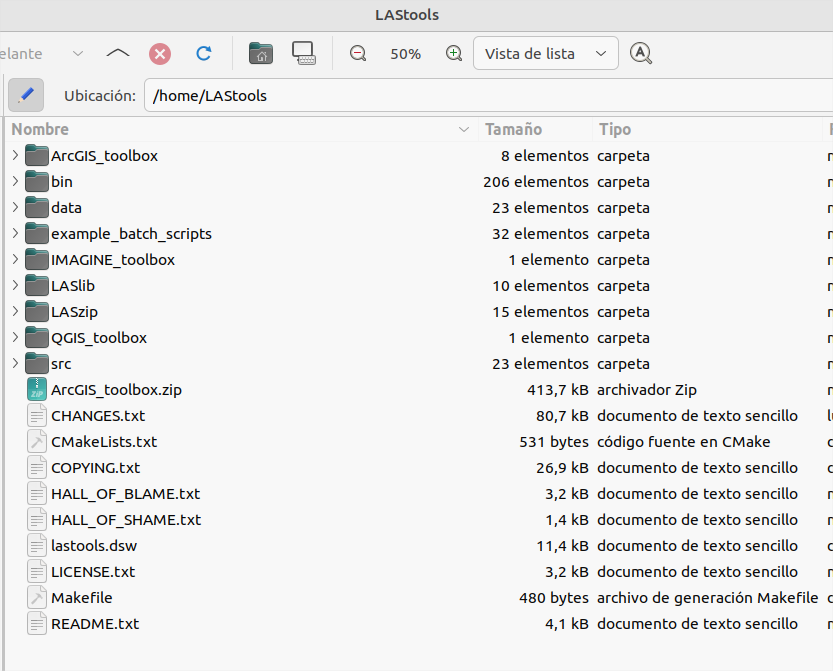
Unzip the compressed .zip file in a simple folder (without spaces or special characters)
Now open QGIS, search in the plugins list for LAStools and install it.
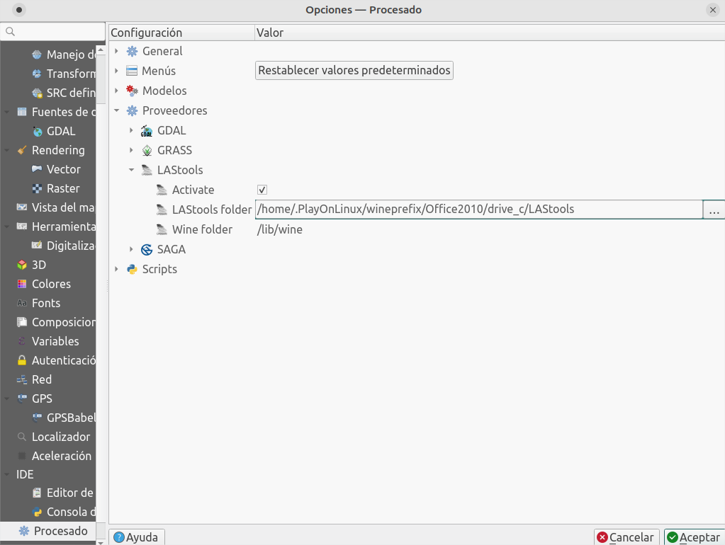
Finally, configure LAStools' installation folder (if it's different from the default C:/ ). The settings shown below work in Linux with Wine installed (using PlayOnLinux in my case).
Extract types of LIDAR data
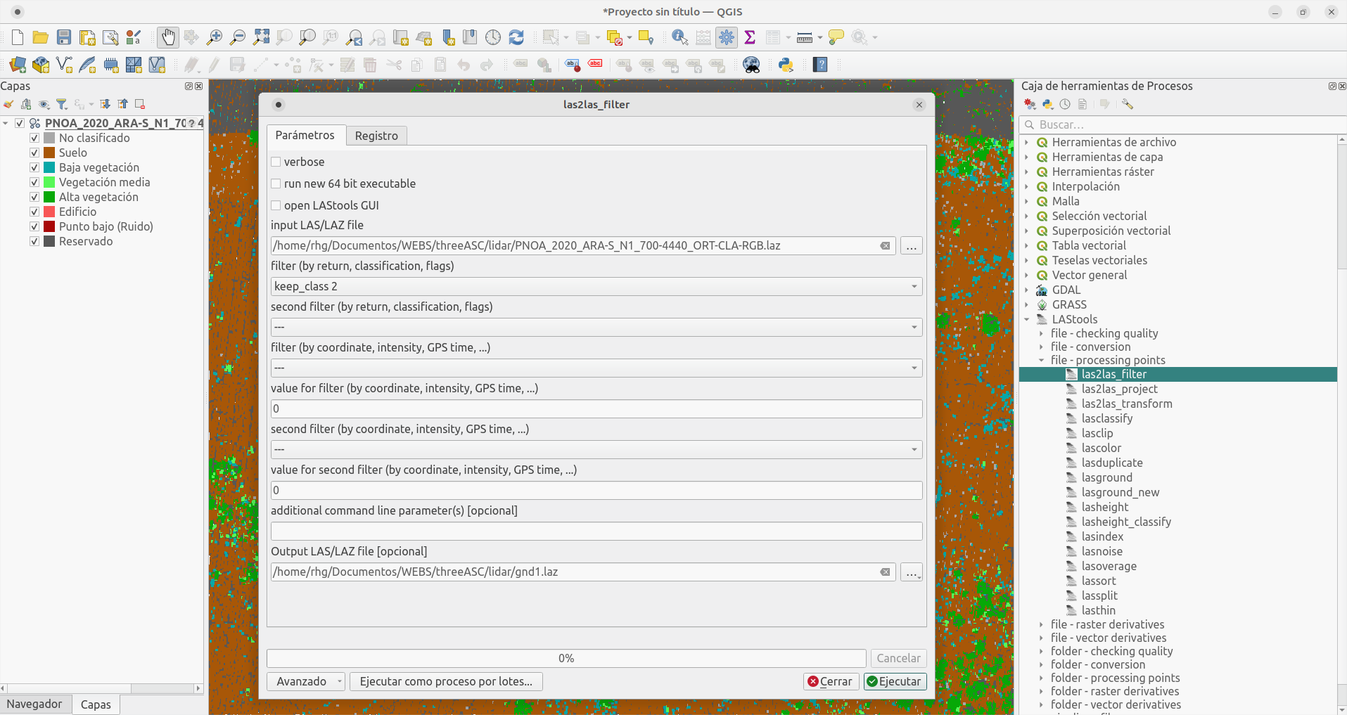
Using LAStools we can extract information of the different data that makes up the point cloud. For example, we'll only extract the data classified as Suelo (soil) which is assigned to a value of 2.
With the process las2las_filter we'll create a filtered point cloud:
Select the .laz file to filter.
On filter, choose the option to keep_class 2
Leave the rest by default, and introduce 0 where the fields require a value
Finally, save the file with .laz extension in a known location to find it easily.
Once finished, just load the generated file and see the point cloud showing only ground data (with buildings and vegetation removed).
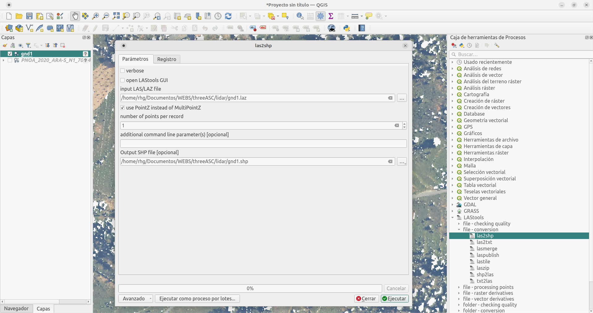
LIDAR to vector conversion
Now use the process las2shp to transform the point cloud into a vector format so you can operate easily with other GIS tools:
Choose the point cloud file just filtered.
Specify 1 point per record to extract every point of the cloud.
Save the file with .shp extension in a known location to find it easily.
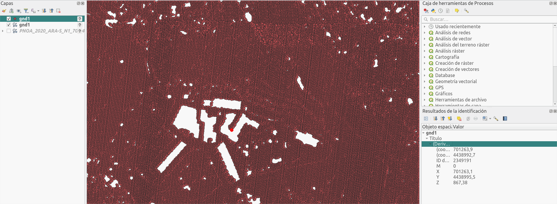
And this will be your filtered point cloud in the classic vector format.
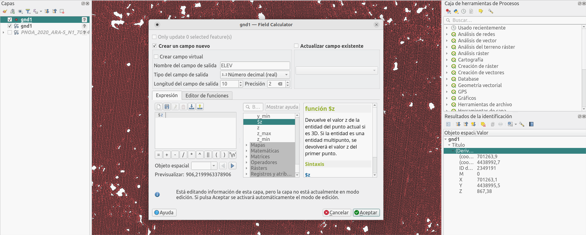
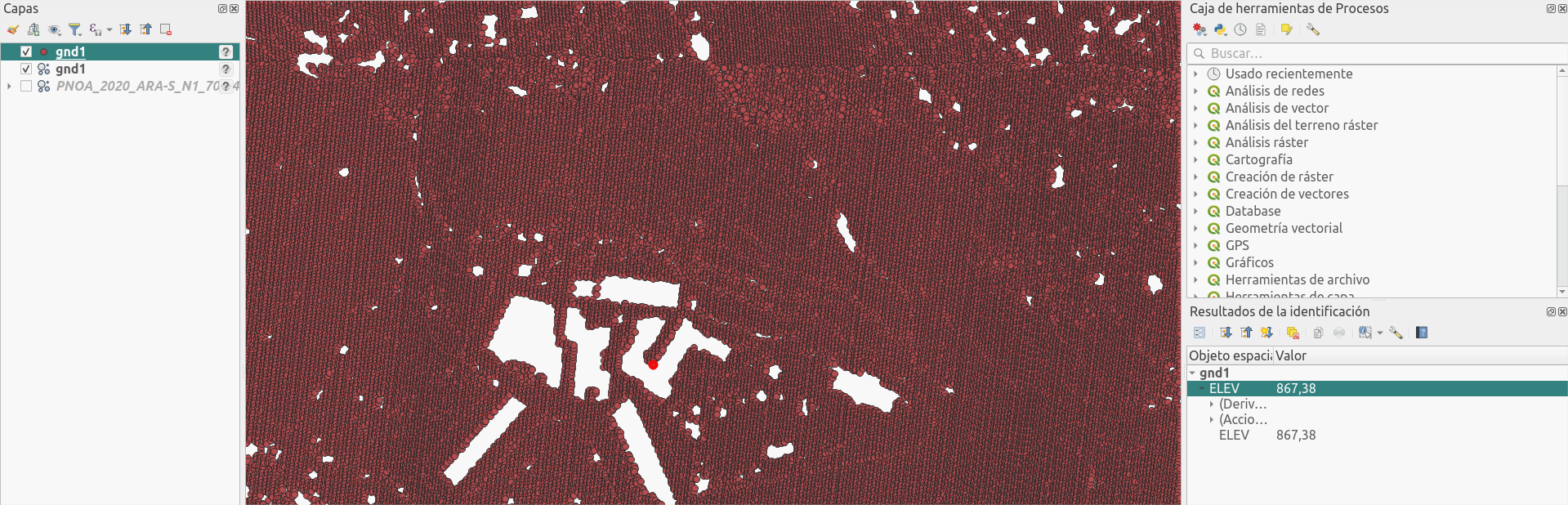
You can see that there is no specific field in the table of attributes. I'll create a new field ELEV to save the Z (height) coordinate and use it to generate a Digital Terrain Model.
3. Digital Terrain Model creation
Raster form vector point layer
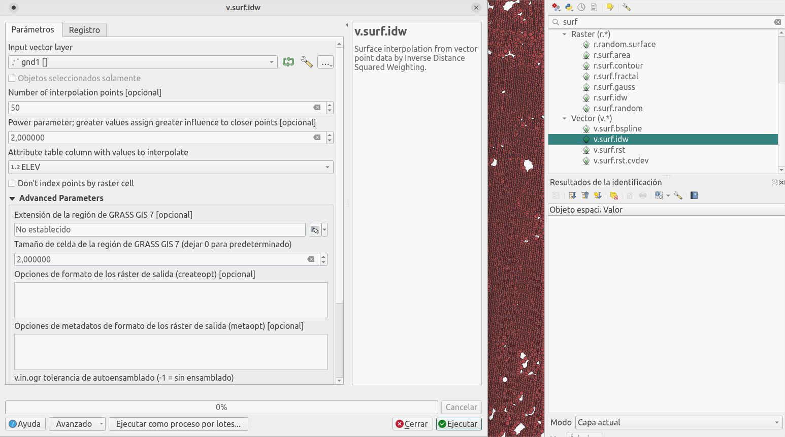
Thanks to the integration of GRASS GIS, we can make use of powerful vector and raster processing tools. Let's use v.surf.idw to generate a regular grid from the interpolation of data in a point layer (in this case the values are weighted with the inverse of the distance but the are other spline algorithms).
Choose the vector point layer.
Choose the number of points to use for interpolation (in this case the data is quite dense so I'll choose 50). The more you choose, the softer the result will be, at the expense of losing the detail of the information density.
Leave the power with the value of 2, to use "square inverse distance".
Choose the data field used in the interpolation (ELEV).
Define the grid cell size. I choose 2 to compare the result with the 2m DTM product from IGN.
4. Result
Let's zoom out and see how it all finished:
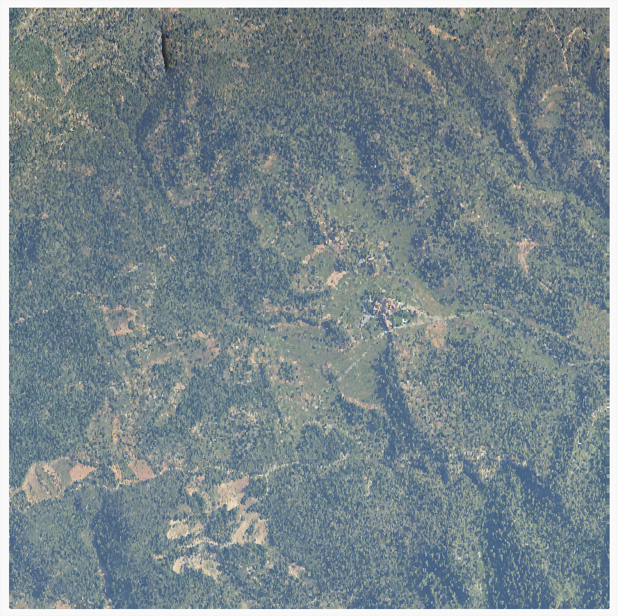
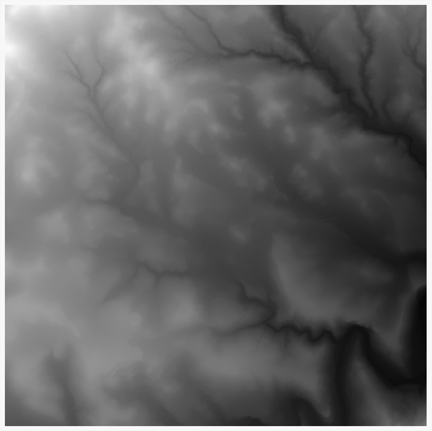
RGB LIDAR point cloud2 meter DTM from LIDAR
And now let's see a bit more detail.
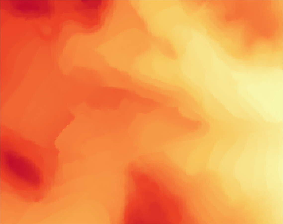
Apply the same color ramp to the generated DTM and to the IGN product. Overall, the result is very similar, with some differences in tree areas, being more reasonable in the processed layer.
MDT 2m LIDARMDT 2m IGNLIDAR + SatIGN + Sat
And that's it! Any doubt or comment can be dropped on Twitter!
If you know my #WarTraces post, you’ll see that I use satellite imagery from the European Space Agency. Today I’ll show how to download and manipulate these images from mission Sentinel 2, as well as Landsat, being very similar to do.
I’ll do it in QGIS, so you need to download this software with the GRASS GIS module included.
Content
Sign up in platforms.
You need to create an account to access both data sources, just filling a form and confirming via email.
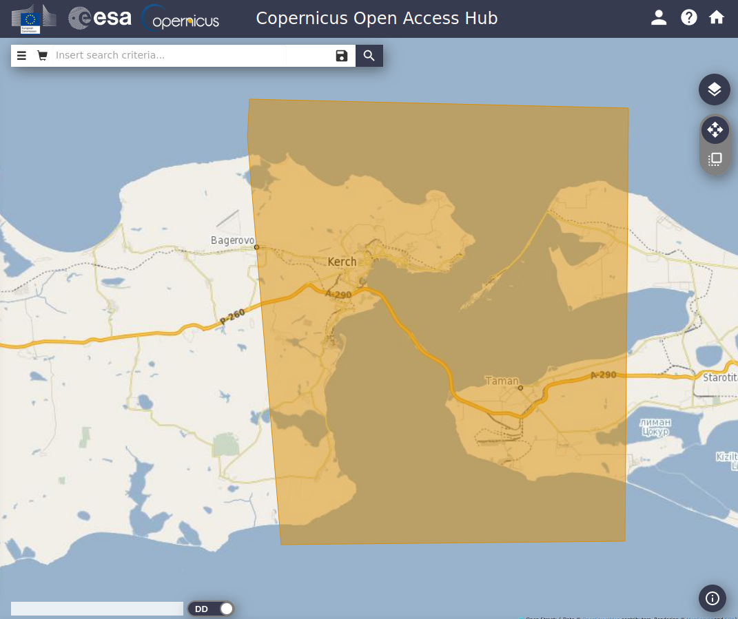
Now, draw a delimiting polygon of the area of interest. Every corner is set with right click, and the polygon is closed with double right click.
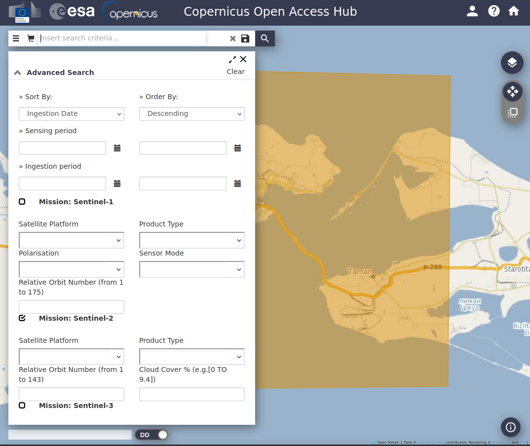
Next, click the filter icon in the search bar and tick the box for mission Sentinel-2 (you can also set dates, but it will be sorted from recent to old by default).
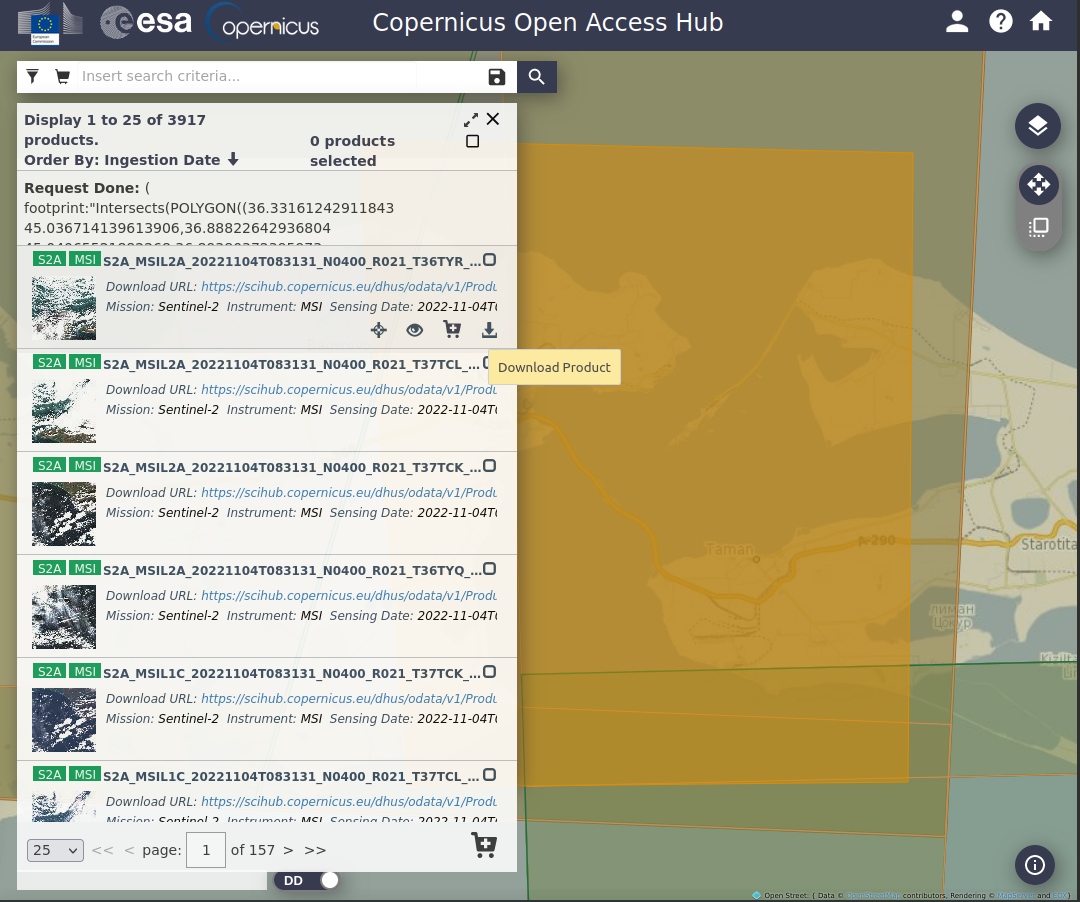
Finally, all available products will appear, so you can preview or download in a compressed .zip file.
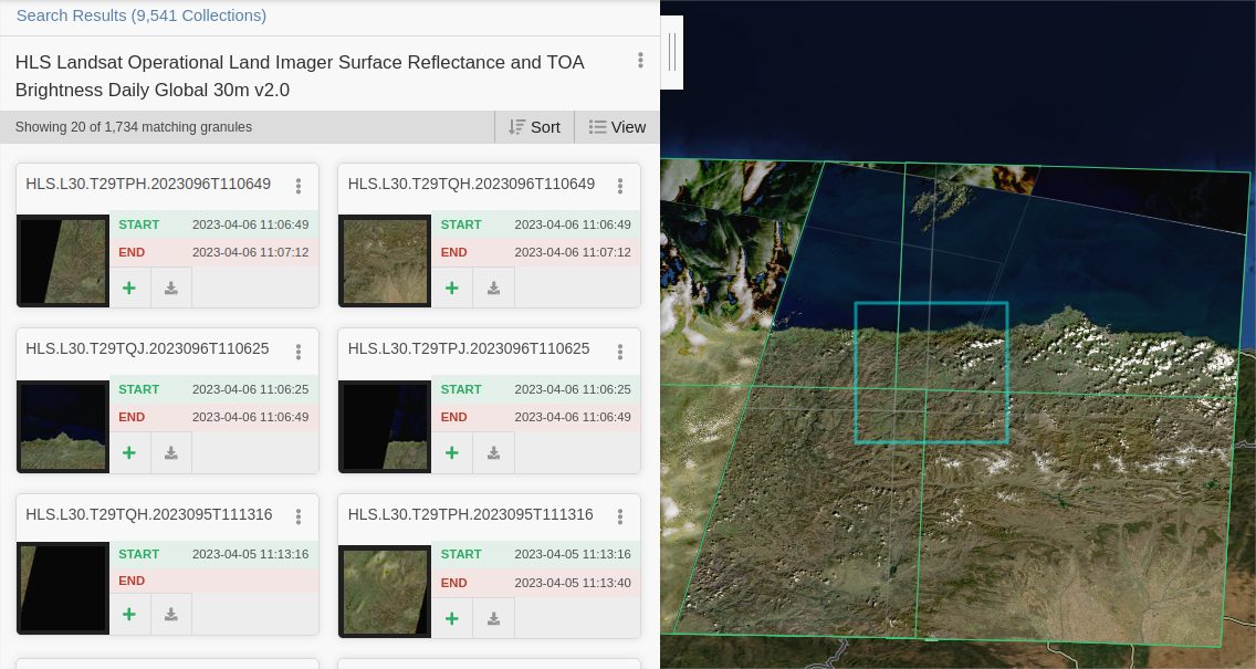
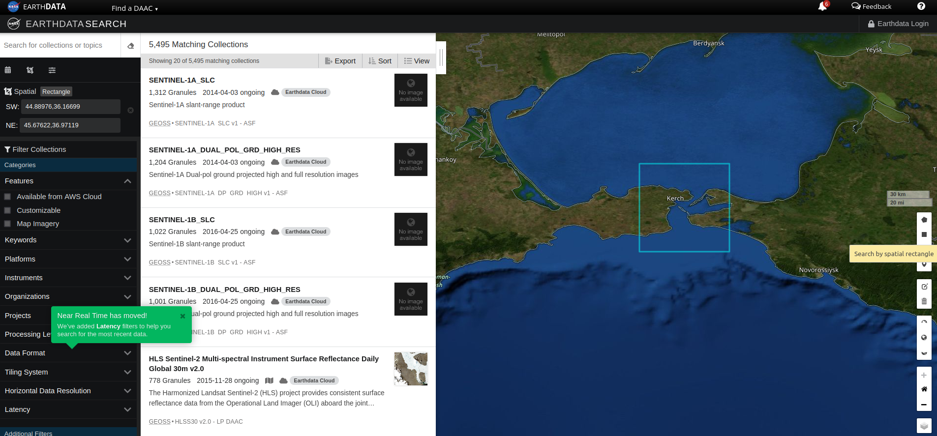
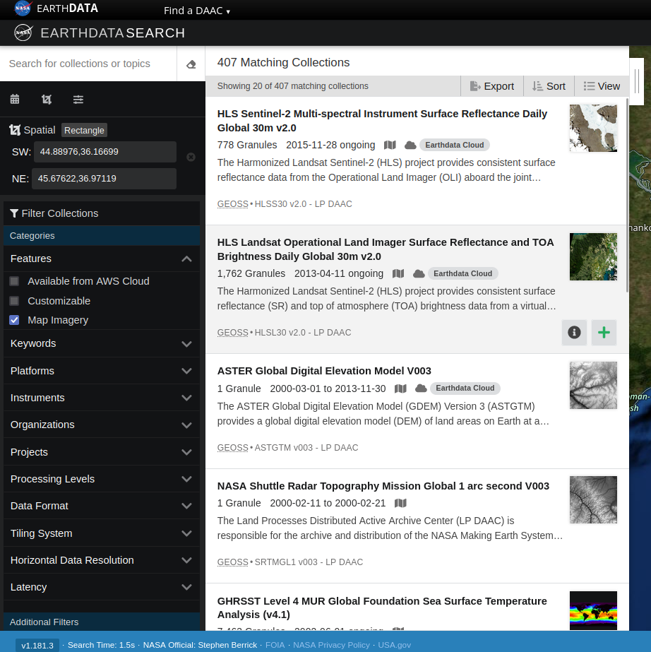
Define an area of interest using the geometry tools in the lateral bar.
Filter the products, for example selecting "Imagery". Then select the HLS Landsat dataset in the catalogue.
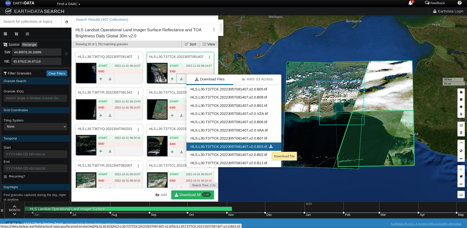
In this case, we need to download each band separately, which we'll see next.
TCI image (true colour)
Simplifying (a lot), satellites capture images in different wave longitude ranges, called bands.
Also, digital images or pictures that we use to represent reality seen by the naked eye use to be defined in three layers: one for color Red, another for color Green, and another one for Blue, defining in each of these layers one value for every pixel with the amount of this color. The combination of all pixels is what simulates an image similar to reality.
TIP! Do the test and zoom in a lot in any picture and see the mosaic of pixels that make it up.
Lets use the bands captured by satellites in the visible wave range to generate an image as if we saw it from space.
Sentinel 2
In the case of Sentinel 2, we can show a true color image directly downloading the product L1C and using the layer _TCI.jp2 located in /GRANULE/DATASET_CODE_NAME/IMG_DATA/
The TCI image will show like this:
Deir ez Zor, Syria, 22/10/2017. TCI. Source: Copernicus Sentinel 2.
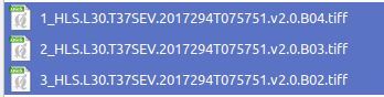
For Landsat, we need to combine the different bands captured individually by the satellite in the visible wave range. These are:
RED
B04
GREEN
B03
BLUE
B02
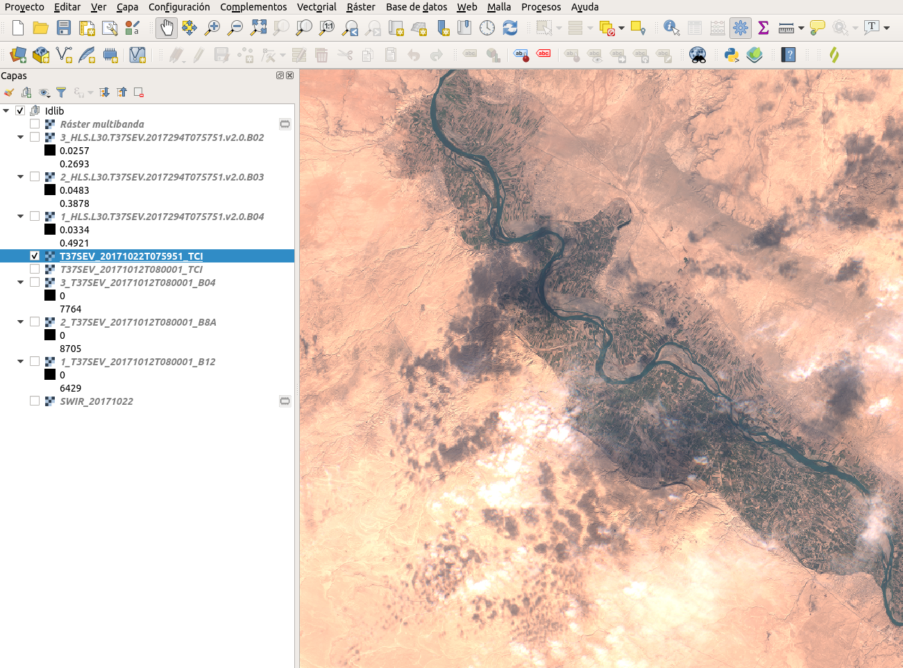
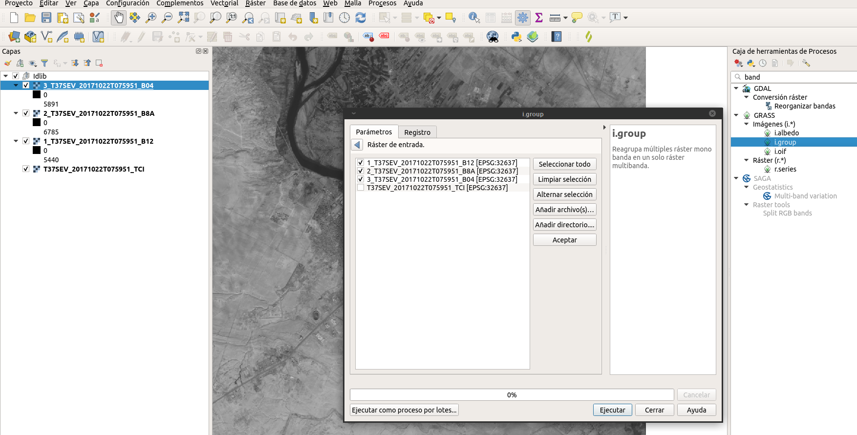
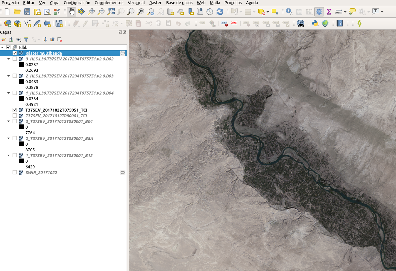
Now in QGIS, we'll use function i.group from GRASS module which combines the selected layers in a multiband Red, Green, Blue layer.
To make it easier, I rename the layers like this, to make sure the script reads them properly:
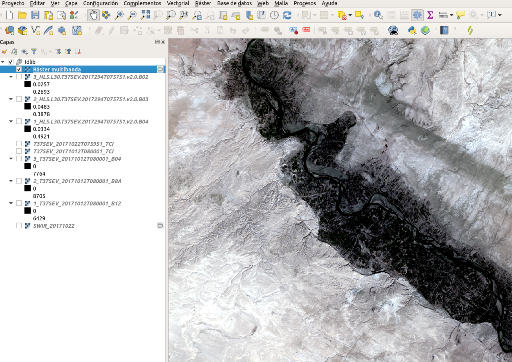
Looking like this:
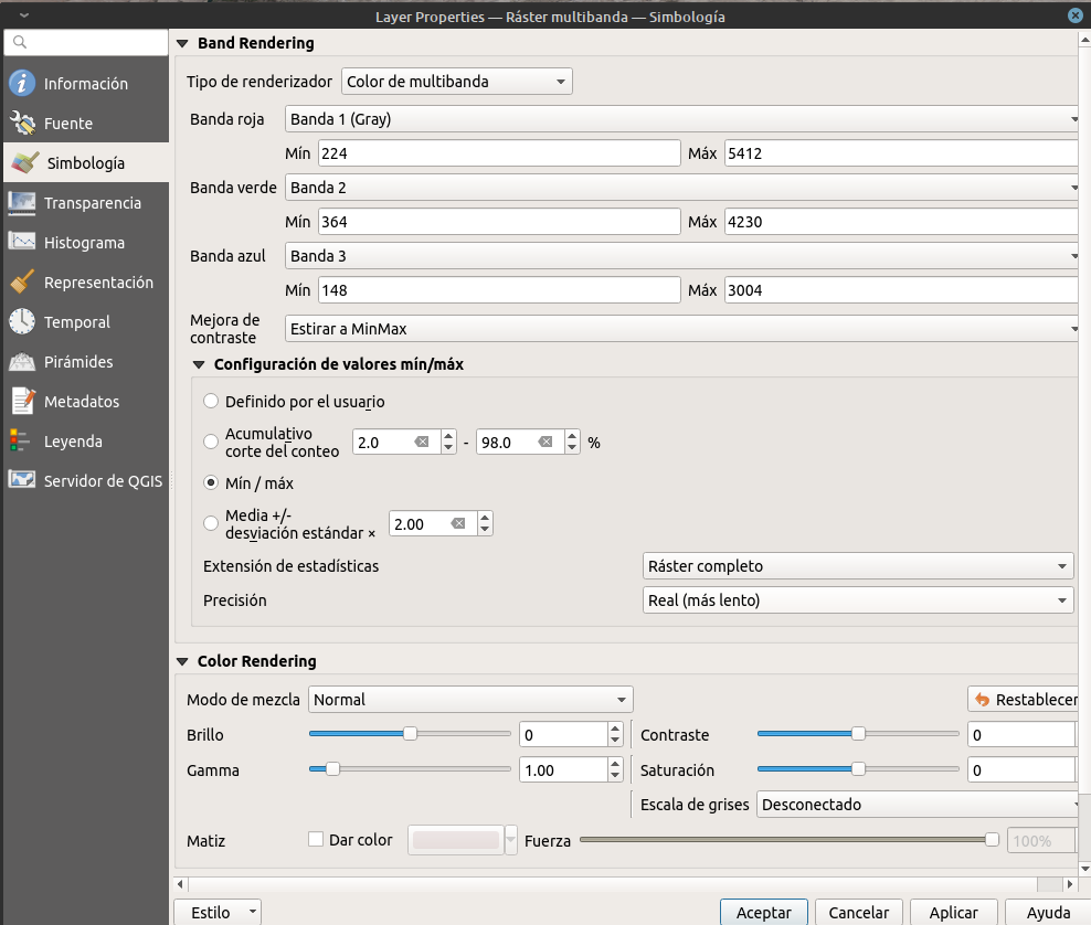
In this case it's nothing similar to the previous image or reality, so we'll adjust the properties to extract more color from the data:
First, let's make sure we use all the data reading real max/min values rather than estimated.
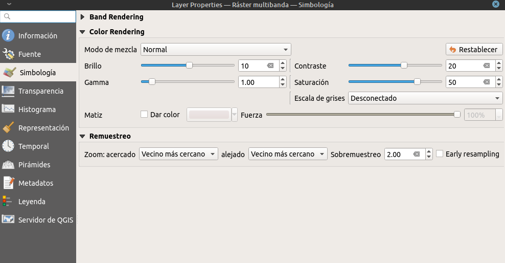
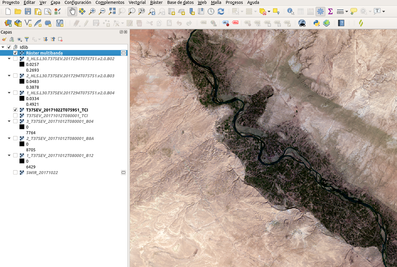
The image already looks better, but missing some brightness and color.
So let's adjust Color Rendering parameters:
And it now looks more realistic:
Deir ez Zor, Siria, 21/10/2017. TCI. Source: Landsat.
SWIR (short wave infra-red)
Using bands in infra-red wave length, we can see further more than with the naked eye, or even across certain objects like some clouds or smoke.
During summer wildfires, I saw how Copernicus used these images to trace the extent of fires, and I thought they could be used to locate bomb impacts under the smoke they produce. That's how this ended in #WarTraces.
Sentinel 2
Using the process above, now we combine the following bands:
RED
B12
GREEN
B8A
BLUE
B04
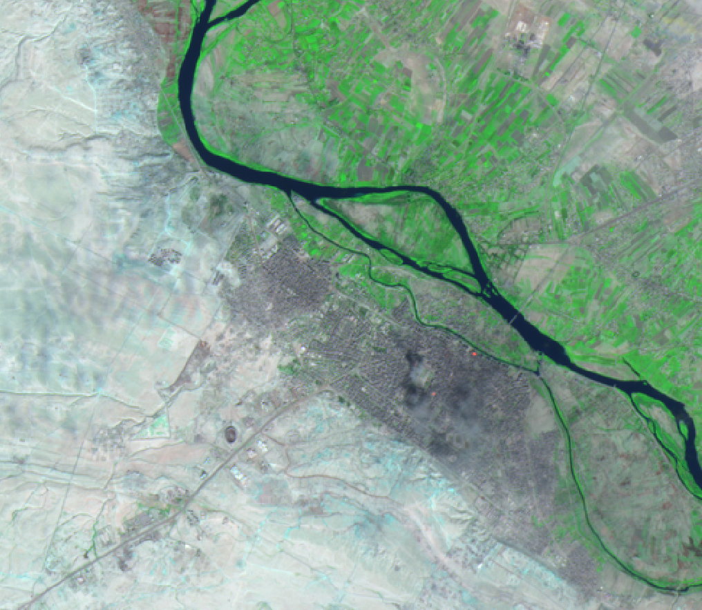
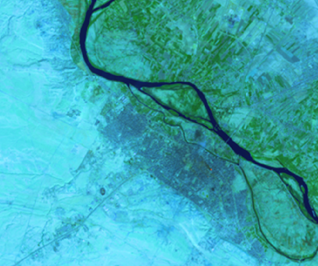
Deir ez Zor, Syria, 22/10/2017. SWIR. Source: Copernicus Sentinel 2.
Landsat
Make a new combination of these bands:
RED
B07
GREEN
B06
BLUE
B04
Deir ez Zor, Syria, 21/10/2017. SWIR. Source: Landsat.
Conclusion
As a final note, it's important to highlight the pixel size, as it will affect image detail (resolution):
Sentinel 2: 10 meters.
Landsat: 30 meters.
On the other hand, Landsat provides images since 2013, while Sentinel only provides data from 2015.
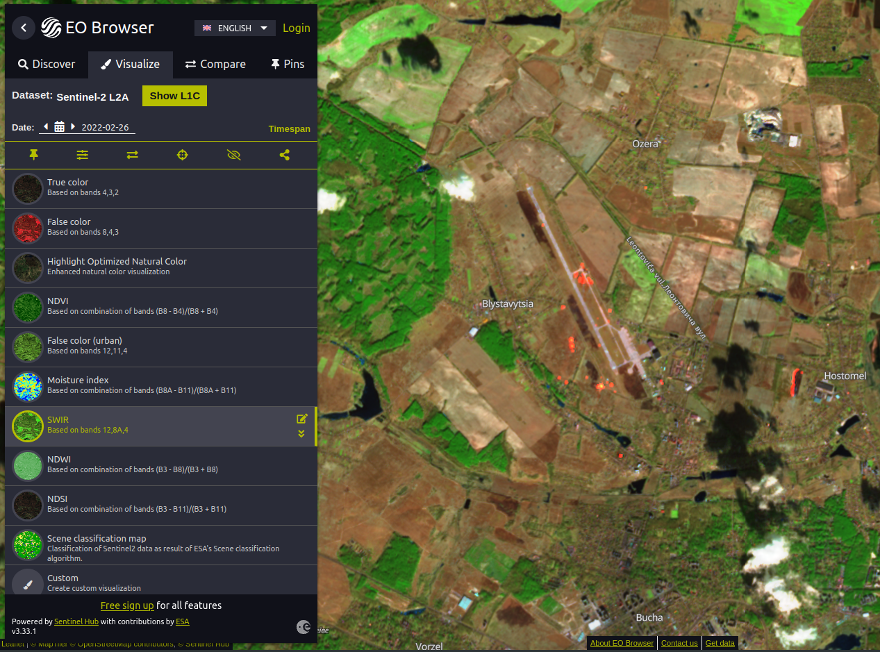
Also, you can preview all these layers and combinations in online viewers like EO Browser by Sentinel Hub.
Bombings in Antonov International Airport, Kyiv, Ukraine, 26/2/2022 using EO Browser.
If you get stuck or want to comment, let me know on 🐦 Twitter!
Blender is (to me), the top free 3D modelling software. It’s got a huge community, tones of documentation, tutorials and, overall, continuous updates and improvement.
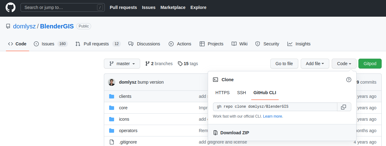
One of the most useful tools is BlenderGIS, an external plugin that lets us drop geographical data, georeferenced or not, and model with them.
Let’s see a use case with an elevation model.
Content
Installation
First thing to do is to download and install Blender from an official source (their website) or from our OS app store:
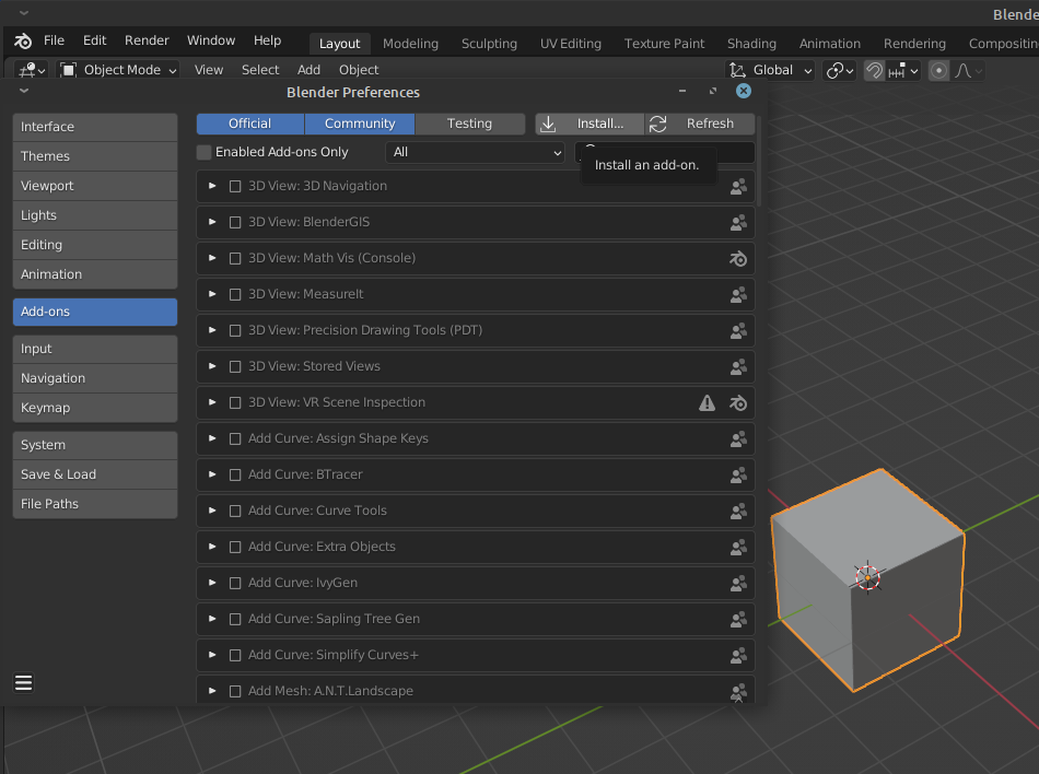
Let's now start Blender and open Add-ons settings (Edit > Preferences > Add-ons).
Press "Install..." and select the BlenderGIS .zip file.
Now you can search it and activate it.
You'll see there's a new "GIS" option in Blender's top bar.
Download geographical information
In this example I will use a Digital Terrain Model in ASCII format (.asc), as it is one of the working formats for BlenderGIS and also the standard for my download source.
If the information you download is in another format, like .tiff or .xyz, you can convert it using some software like QGIS or ArcGIS.
MDT
In my case, I will use MDT200 from spanish IGN, a terrain model with 200m cell size, as I want to show quite a large area that includes the province of Álava.
We can also use an orthophoto as a terrain texture. For this, I will be using QGIS and I will load a WMS also from IGN so I can clip the satellite image exactly to the terrain tile extent.
Load the orthophoto and the terrain layers, then export the orthophoto layer as a rendered image and set the extension from the terrain layer. I will set the cell size to 20 meters (although the imagery allows up to 20cm cell size, which would result in a huge file; the 20m image is already 140MB).
TIP! One way to optimize detail is to generate a grid of smaller size images but higher resolution.
Modelling in Blender
Now it's all ready for Blender.
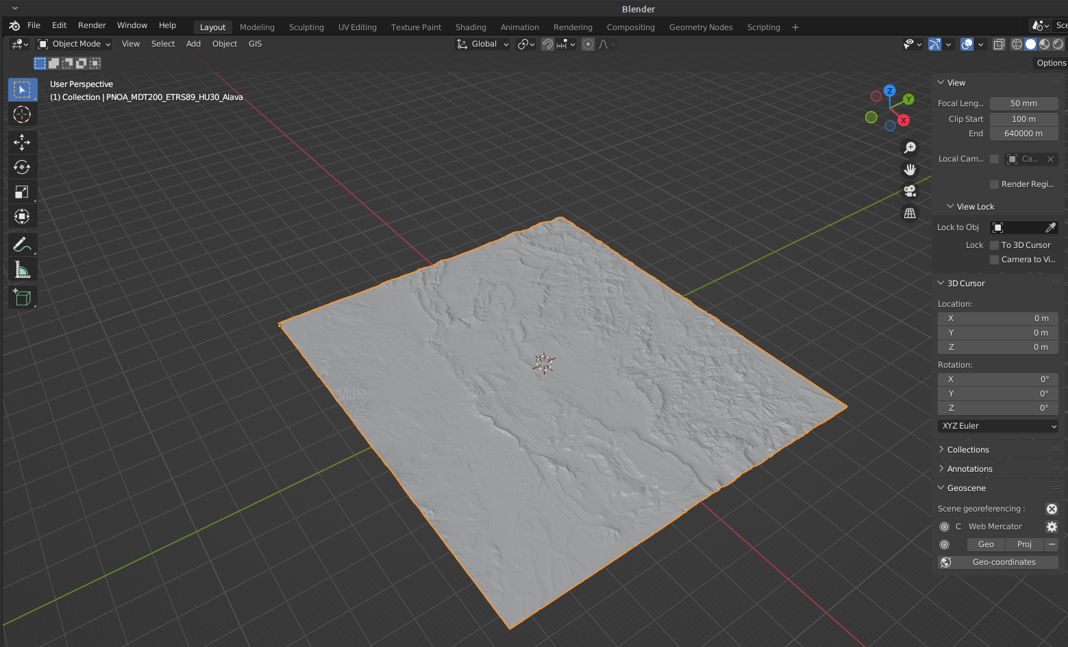
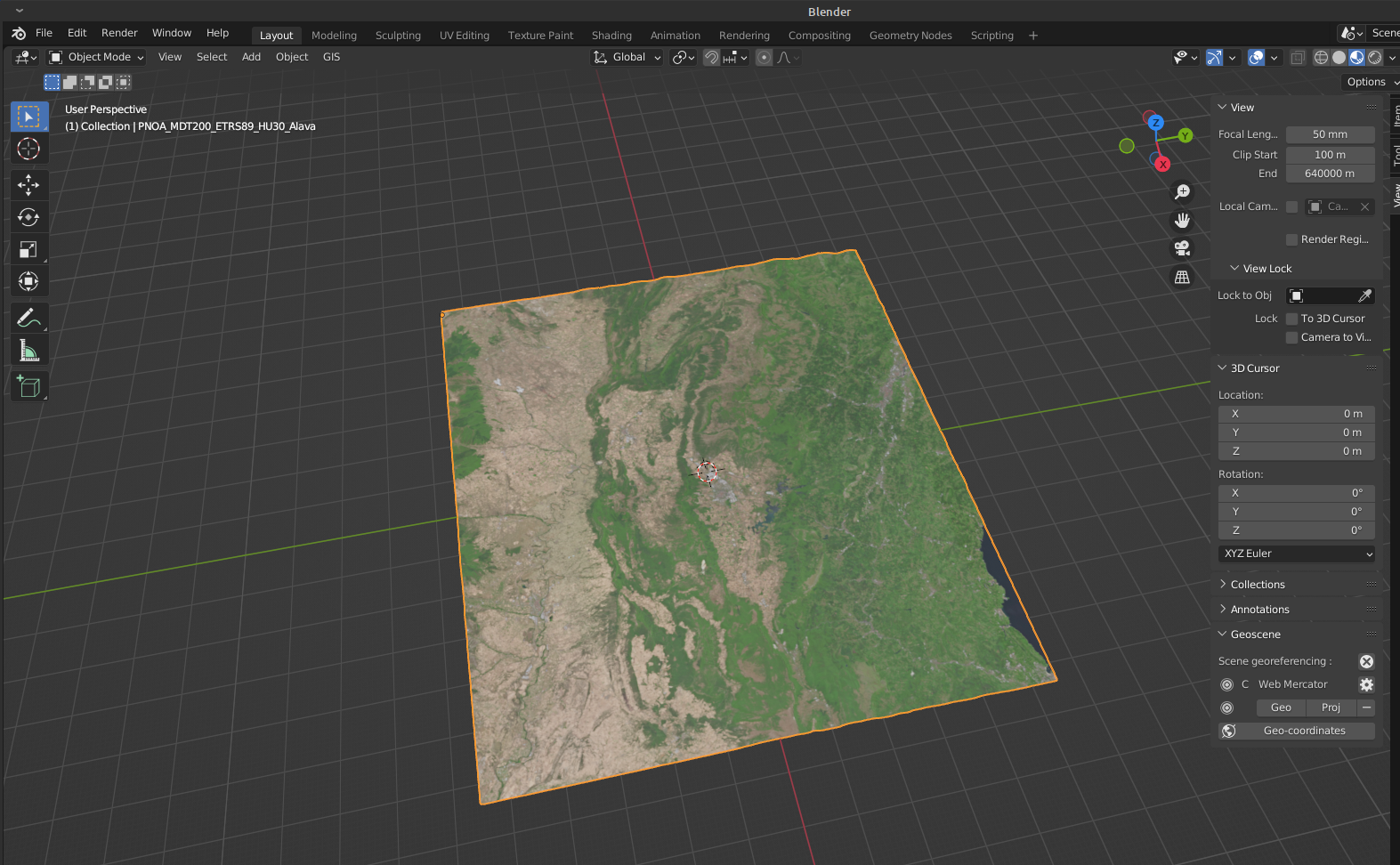
Using the "GIS" menu, import the terrain layers as an ASC grid. You'll see it quickly shows up on screen.
TIP! This model is centered in coordinate origin, but you can georeference the model setting a CRS in the "Geoscene" properties.
Let's add the satellite image:
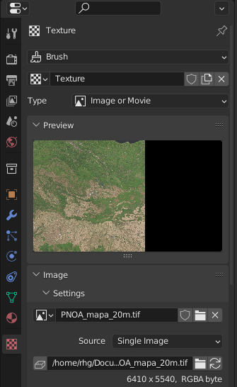
Create a new material.
Create a new texture and load the satellite image.
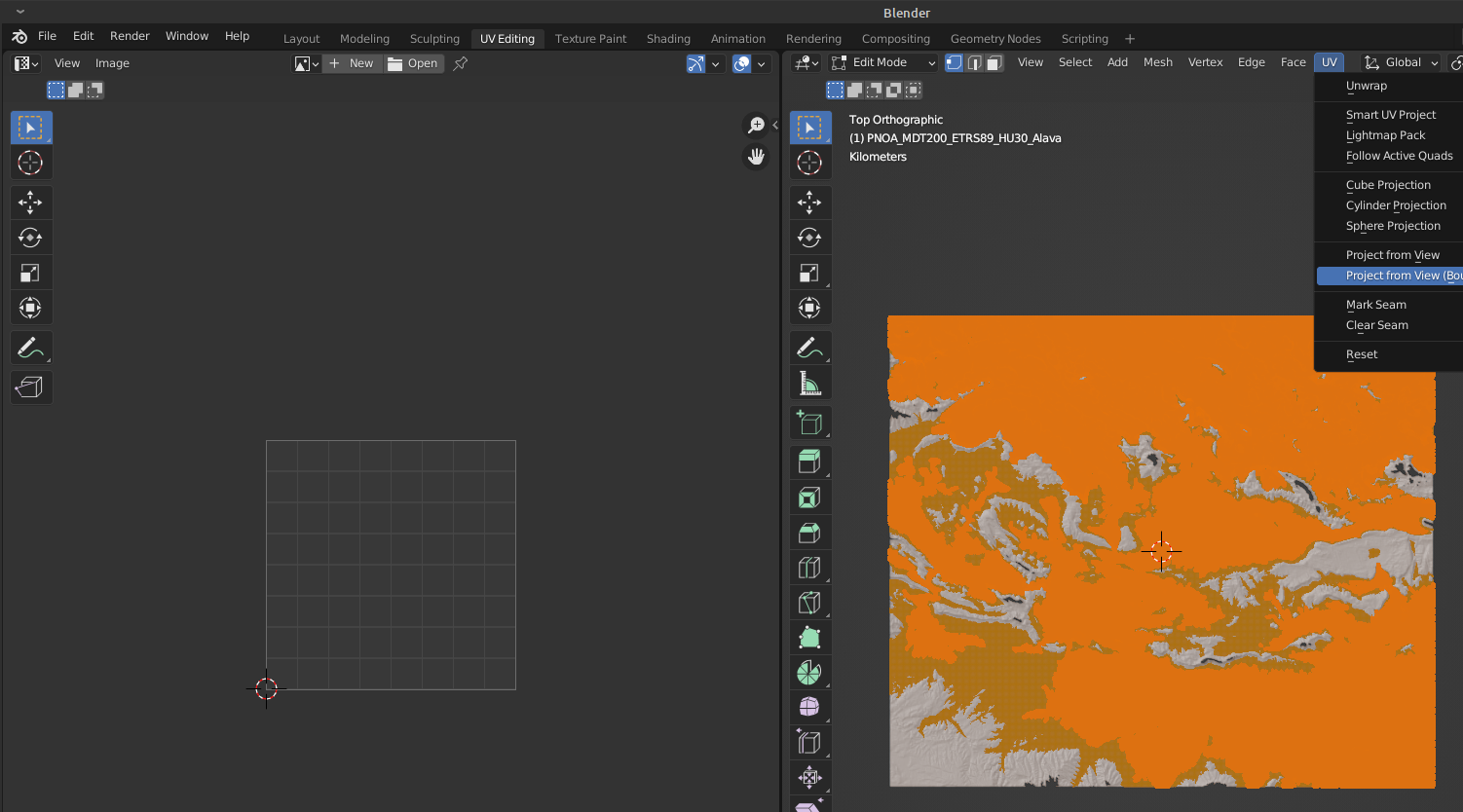
Now move to UV Editing tab.
Select the terrain layer on the right window, enter Edit Mode, and "Select all" faces (Ctrl+A). You should see it orange as below and make sure you are in "Top" view (press number 7).
Click on "UV" tools in the top menu and project the terrain layer with "Project from View (bounds)". This makes it fit the image extent.
On the left window, choose the image texture to apply to the projection and see how the grid adjusts to it (try making zoom on it)
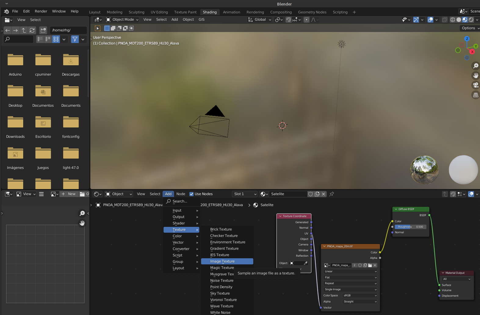
Finally, go to the Shading tab and add the element "Image Texture", choosing the right image and connecting Vector to UV and Color to Shader (just copy the image below).
If you now go to the Layout window, the model will show the satellite image perfectly adjusted.
And it's ready so you can edit and export your model, for example, for 3D printing or for a realistic Unity3D scene.
If you’ve used desktop GIS software, you will be surprised that many geospatial tools are also available to use in your web maps using a free and open-source javascript library.
Today I show you TurfJS. Press the button 🌤 in the map below and see one of many possibilities: inverse distance weighting or IDW.
Content
Installation
TurfJS hosts a practical website explaining all available functions, as well as the initial setup:
markers.forEach(function(m){
    var marker=L.marker([m.lat, m.lon]).addTo(map);
    marker.bindTooltip("<b>"+m.name+"</b><br>"+m.dato).openTooltip();
});

//WE ADDED A SINGLE MARKER LIKE THIS ON LEAFLET
//var marker = L.marker([25.77, -80.13]).addTo(map);
//marker.bindTooltip("<b>Estacion1</b><br>m.dato").openTooltip();
//empty points array
var points=[];

//loop to fill the array with data
markers.forEach(function(m){
    points.push(turf.point([m.lon, m.lat],{name: m.name, dato: m.dato}));
});

//convert to Turf featureCollection
points=turf.featureCollection(points);
TIP! Note that Turf taked coordinates as longitude-latitude, instead of the usual latitude-longitude!
Define interpolation options, having the following:
gridType: or cell shape
points
square
hex
triangle
property: field that contains the interpolation values.
units: spatial units used in the interpolation:
miles
kilometers
radians
degrees
weight: power used in the inverse distance weighting, usually 2, although higher values will make a smoother result.
//interpolation options: rectangular grid using 'dato' variable in kilometers using the power of 2

var options = {gridType: 'square', property: 'dato', units: 'kilometers', weight: 2};
Finally, generate the interpolated grid and add it to the map, being the numeric value the cell size of the grid (0.5 Km):
//create Turf grid
var malla=turf.interpolate(points, 0.5, options);

//add to Leaflet
L.geoJSON(malla).addTo(map);
Generating this result (nothing conclusive):
Format grid and show values
Seems not, but the interpolation is done, it's just shown incorrectly.
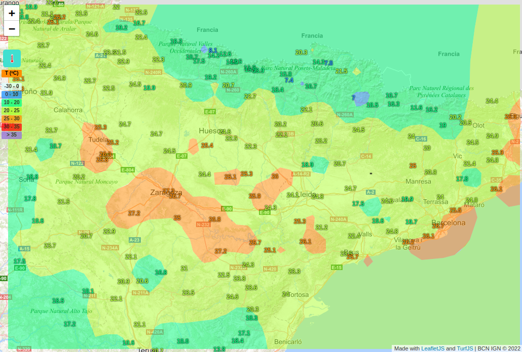
I'll add a color ramp to represent data, and also show values when hovering the cells. Let's modify the Leaflet geoJSON object properties for this:
style: function to modify object style, according to its value.
onEachFeature: function added to each object to interact with it.
Let’s now pay attention to the detail of the API and how to access all the available data.
Content
API access
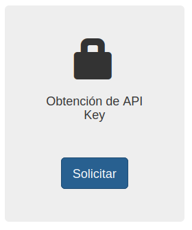
To use the API we need an API key. Go to the AEMET OpenData webpage and click on "Solicitar" to request it.
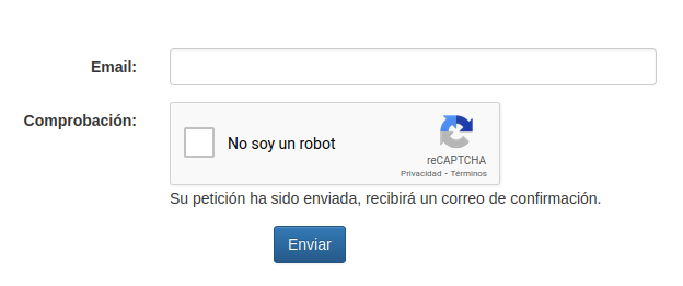
Next we'll be asked for an email address where the key will be sent.
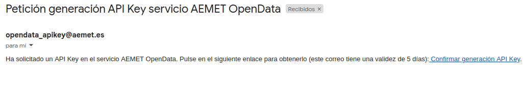
You'll receive a first confirmation email, and then a second email with the access key. Let's copy it and keep moving.
Documentation and examples
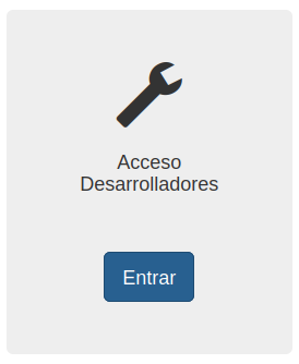
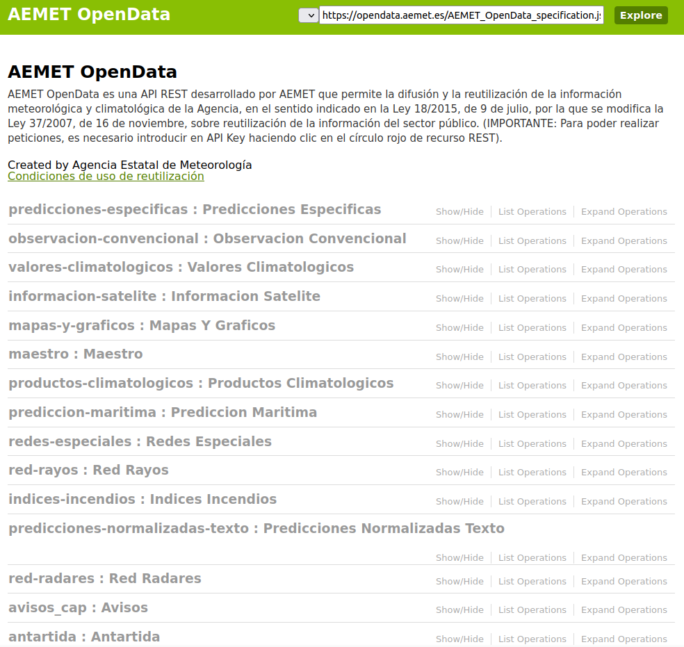
Get back to AEMET OpenData and into the developer's section "Acceso Desarrolladores".
We're interested in the dynamic documentation, which shows all the data requests available that we can try live.
Click on each topic to display the syntax for every data request.
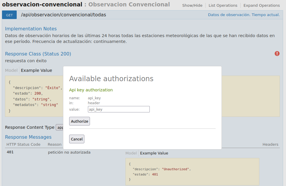
Click on observación-convencional and then /api/observacion/convencional/todas.
Now click on the red sign on the right, where you'll paste and authorize the API key.
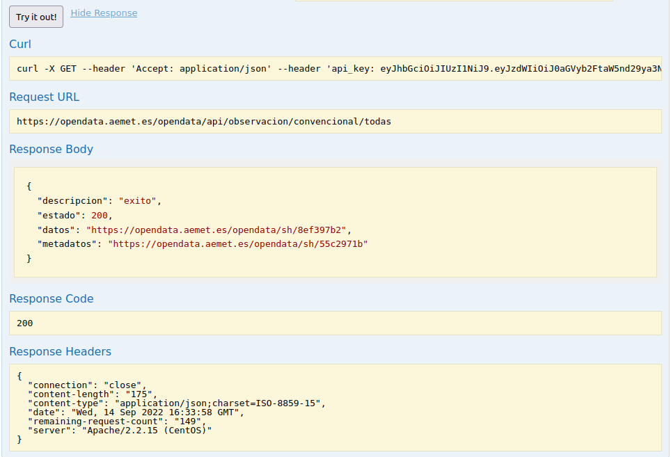
Now press the Try it out! button and you'll get:
a curl request example
the request URL
the body, code and headers of the response
If we open the URL inside the "datos" field we'll see the full list of data for all the stations. A JSON lot like this:
Loading...
The main fields are the following:
idema: station ID or code.
lat and lon: latitude and longitude coordinates.
alt: station altitude.
fint: data interval date.
prec: precipitation in this period.
vv: wind speed in the station.
ta: ambience temperature in the station.
Data request using javascript
HTML structure
I'll develop an example to access the data and make use of them.
I'll simply create a .html document with a request button, a text line and a request function:
Click the button to request data
<html>
<body>
<button id="solicitud" onclick="solicitar()">Request</button>
<p id="texto">Click the button to request data</p>
</body>
<script>
function solicitar(){
document.getElementById("texto").innerHTML="I didn't program that yet..";
}
</script>
</html>
TIP! Copy and paste the code above in a text document with .html extension and open it in your browser.
HTTP request
We'll do the data request in javascript using the XMLHttpRequest object. The example from w3schools is really simple:
As we saw in the dynamic documentation, after doing the request, we got a link to the data, which is another request, no we need to nest two requests like this:
<script>
function solicitar(){
// Define loading message
document.getElementById("texto").innerHTML="Cargando datos...";
// Define API Key
var AK=tUApiKey;
// Define request URLs
var URL1="https://opendata.aemet.es/opendata/api/observacion/convencional/todas";
var URL2="";

// Create XMLHttpRequest objects
const xhttp1 = new XMLHttpRequest();
const xhttp2 = new XMLHttpRequest();

// Define response function for the first request:
// We want to access te "datos" URL
xhttp1.onload = function() {
  // 1º Parse the response to JSON:
  URL2=JSON.parse(this.responseText);
  // 2º Get the "datos" field:
  URL2=URL2.datos;
  // 3º Make the new request:
  xhttp2.open("GET", URL2);
  xhttp2.send();
}

// Define response function for the second request:
// We'll modify the text line with some information in the data
xhttp2.onload = function() {
  // 1º Parse the response to JSON (much better to work with):
  var datos=JSON.parse(this.responseText);

  // 2º Get the length of the JSON data
  // This is equivalent to the individual hourly entries per stations
  var registros=datos.length;

  // 3º Get first entry date.
  // We'll format it as it's in ISO standard
  var fechaini=datos[0].fint;
  fechaini=new Date(fechaini+"Z");
  fechaini=fechaini.toLocaleDateString()+" "+fechaini.toLocaleTimeString();

  // 4º Get last entry date.
  // We'll format in the same way
  var fechafin=datos[(datos.length-1)].fint;
  fechafin=new Date(fechaini+"Z");
  fechafin=fechafin.toLocaleDateString()+" "+fechafin.toLocaleTimeString();

  // 5º Merge it all and display in the text line
  document.getElementById("texto").innerHTML="Se han descargado <b>"+registros+"</b> registros desde el <b>"+fechaini+"</b> hasta el <b>"+fechafin+"</b>. <a href='"+URL2+"' target='_blank'>Ver todos los datos.</a>";
}

// Send the first request
xhttp1.open("GET", URL1+"/?api_key="+AK);
xhttp1.send();

}
</script>
Let's see the result below:
Click the button to request data
And done! This way you can obtain coordinates and values for different metheorological stations from AEMET and drop them in a table or web map like we've seen for Leaflet here.
The usual way to see and work with these files is using a GIS software like QGIS or ArcGIS, but how can we make this friendly to standard users? Wouldn’t it be better seen directly in 3D and visit the place virtually?
At this point is where I found CesiumJS: a 3D map viewer styling [G] Earth but open-source, free and highly customizable to make your own projects.
CesiumJS demo viewer of the new Tajogaite terrain with IDE Canarias satellite imagery. Click on the map to interact or open the full version.
Content
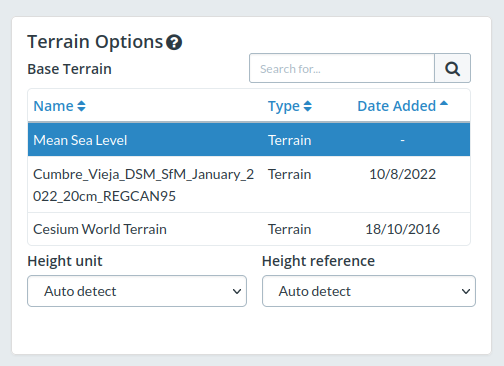
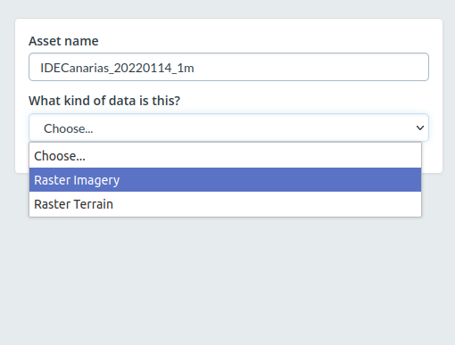
Create a Cesium ion account
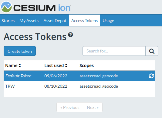
To use CesiumJS you need to register an account in order to obtain an Access Token.
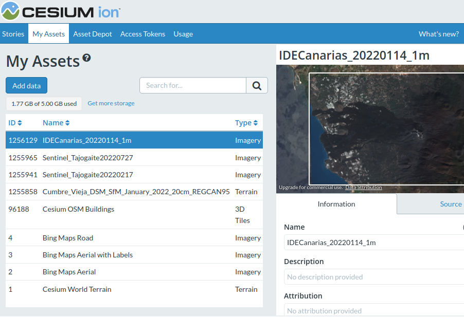
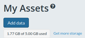
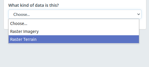
Registering, we can also upload our own files to customize our 3D map creations. In my case you can see that I uploaded the Digital Surface Model and imagery of the viewer. I drop the links in case you want to use the same files:
TIP! You can use the WMS service in your GIS software to extract the imagery, or download the one I use in this example (270 MB with 1m resolution)
Include CesiumJS in your web.
To use CesiumJS we configure a .html file as usual.
In this case, I'll copy the code directly from their quickstart example as it is only about 25 lines:
As you see, the main parts are:
links to CesiumJS libraries in the <head>
a <div> element with id "cesiumContainer" inside the <body>
the Access Token as variable Cesium.Ion.defaultAccessToken. Introduce yours here.
a "viewer" variable
the initial viewer configuration, specifying initial coordinates and X, Z angles.
<!DOCTYPE html>
<html lang="en">
<head>
  <meta charset="utf-8">
  <!-- Include the CesiumJS JavaScript and CSS files -->
  <script src="https://cesium.com/downloads/cesiumjs/releases/1.97/Build/Cesium/Cesium.js"></script>
  <link href="https://cesium.com/downloads/cesiumjs/releases/1.97/Build/Cesium/Widgets/widgets.css" rel="stylesheet">
</head>
<body>
  <div id="cesiumContainer"></div>
  <script>
    // Your access token can be found at: https://cesium.com/ion/tokens.
    // This is the default access token from your ion account
    Cesium.Ion.defaultAccessToken = 'eyJhbGciOiJIUzI1NiIsInR5cCI6IkpXVCJ9.eyJqdGkiOiI1MTYwNGM0Yi1iYzlkLTRkMTUtOGQyOS04YjQxNmUwZDQ0YjkiLCJpZCI6MTA0Mjc3LCJpYXQiOjE2NjAxMDk4MzR9.syNWeKPLWA2eMrEh4K9hvkyp1oGdbLMaL0Ozk1kaksk';
    // Initialize the Cesium Viewer in the HTML element with the `cesiumContainer` ID.
    const viewer = new Cesium.Viewer('cesiumContainer', {
      terrainProvider: Cesium.createWorldTerrain()
    });
    // Add Cesium OSM Buildings, a global 3D buildings layer.
    const buildingTileset = viewer.scene.primitives.add(Cesium.createOsmBuildings());
    // Fly the camera to San Francisco at the given longitude, latitude, and height.
    viewer.camera.flyTo({
      destination : Cesium.Cartesian3.fromDegrees(-122.4175, 37.655, 400),
      orientation : {
        heading : Cesium.Math.toRadians(0.0),
        pitch : Cesium.Math.toRadians(-15.0),
      }
    });
  </script>
 </div>
</body>
</html>
<html lang="en">
<head>
<meta charset="utf-8">
<script src="https://cesium.com/downloads/cesiumjs/releases/1.96/Build/Cesium/Cesium.js"></script>
<link href="https://cesium.com/downloads/cesiumjs/releases/1.96/Build/Cesium/Widgets/widgets.css" rel="stylesheet">
</head>
<body style="margin:0;width:100vw;height:100vh;">
<div style="height:100%;" id="cesiumContainer"></div>
<script>
// Your access token can be found at: https://cesium.com/ion/tokens.
// Replace `your_access_token` with your Cesium ion access token.
Cesium.Ion.defaultAccessToken = 'eyJhbGciOiJIUzI1NiIsInR5cCI6IkpXVCJ9.eyJqdGkiOiI1MTYwNGM0Yi1iYzlkLTRkMTUtOGQyOS04YjQxNmUwZDQ0YjkiLCJpZCI6MTA0Mjc3LCJpYXQiOjE2NjAxMDk4MzR9.syNWeKPLWA2eMrEh4K9hvkyp1oGdbLMaL0Ozk1kaksk';
// Initialize the Cesium Viewer in the HTML element with the `cesiumContainer` ID.
const viewer = new Cesium.Viewer('cesiumContainer', {
//terrainProvider: Cesium.createWorldTerrain()//terreno original
terrainProvider: new Cesium.CesiumTerrainProvider({//terreno modificado
url: Cesium.IonResource.fromAssetId(1255858),
}),
});
// Esconder widgest inferiores
viewer.timeline.container.style.visibility = "hidden";
viewer.animation.container.style.visibility = "hidden";
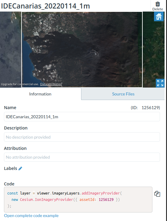
// Add Sentinel2 imagery
const layer = viewer.imageryLayers.addImageryProvider(
new Cesium.IonImageryProvider({ assetId: 1256129 })
);
// Add Cesium OSM Buildings, a global 3D buildings layer.
const buildingTileset = viewer.scene.primitives.add(Cesium.createOsmBuildings());
// Fly the camera to San Francisco at the given longitude, latitude, and height.
viewer.camera.flyTo({
    destination : Cesium.Cartesian3.fromDegrees(-17.8195, 28.6052, 3000),
    orientation : {
    heading : Cesium.Math.toRadians(-85.0),
    pitch : Cesium.Math.toRadians(-30.0),
    }
});
</script>
</div>
</html>
And that's it! You can create tons of immersive web apps with detailed terrains better than the standard ones.
Where else can you use CesiumJS? Tell it on Twitter 🐦
UPDATE 2023! Hourly WMS service removed and daily version updated to V2. WMS version updated to 1.3.0
Recently it’s been trendy to talk about the increased warming of the Sea, and I’ve found very few maps where you can actually click and check the temperature it pretends to indicate.
So I’ve done my own:
I’m going to find a WMS with the required raster information,
Replicate the legend using html <canvas> elements,
And obtain the temperature value matching the pixel color value.
Content
The data
There are several and confusing information sources:
Puertos del Estado: My first attempt was to check the Spanish State Ports website, but the only good thing I found was that they use Leaflet.. They have a decent real-time viewer, but it's really complicated to access the data to do something with them (although I'll show you how in the future).
Copernicus: "Copernicus is the European Union's Earth observation programme", as they indicate in their website, and they gather the majority of geographical and environmental information produced in the EU member countries. In their marine section we'll find Sea Surface Temperature (SST) data obtained from satellite imagery and other instruments from different euopean organisms.
Global Ocean OSTIA Diurnal Skin Sea Surface Temperature
After trying them all, the most complete is the global map produced by the MetOffice.
As they indicate, it shows the hourly average in a gap-free map that uses in-situ, satellite and infrared radiometry.
The basemap
I'll create a basemap as I've shown in other posts.
I'll download it in geoJSON format and convert it into a variable called "countries" in a new file CNTR_RG_01M_2020_4326.js . I need to insert the following heading so it's read correctly (cole the JSON variable with "]}" so it's read correctly).
We'll add the GeoServer functions "?service=WMS&request=GetCapabilities" which will show the available information in the WMS like layers, legends, styles or dimensions.
Find the options values that you need in the metadata file. Specifically these tags:
<Layer queryable="1"><Name> will show the layer names that we can introduce in the proeprty "layers:"
<Style><Name> will show the name for the different styles available to represent the raster map and we'll introduce it in the property "styles:".
<LegenURL> shows a link to the legend used for that style.
<Dimension> will show the units that we can use when querying the WMS. In this case it's a time unit as we can vary the date that the map represents. I'll comment it for the moment so it will show the last available date.
SST raster data
Finally, let's add the legend to the map to have a visual reference.
It's inserted as an image in the <body> and some CSS in <style>:
As you can see, it's hard to try and figure out a value for any of the pixels in the map.
Mimic the legend to query the data
To know the temperature that a pixel represents, we should know the position of such pixel color in the legend, and its proportional value compared to the extreme values (310kPa= 36.85ºC y 210kPa=-3.15ºC).
The problem is that CORS policy won't let you query the image as it's outside our domain. On the other hand, if we add the image to our domain, it will have a low resolution and lose precision in the colors that it shows.
That's why I'll mimic the legend using a <canvas> element.
Using javascript, and the HTML Color Picker, we'll define the different color stops in a "gradient" type fill that will replace the original legend.
	function grad(){
		//Generamos la leyenda en el canvas 'gradientC'
		var ctx=document.getElementById("gradientC").getContext('2d');
		//Definimos un gradiente lineal
		var grd=ctx.createLinearGradient(0,150,0,0);
		//Calibrar las paradas del gradiente tomando muestras de la imagen
		//Descomentar la imagen que va junto al canvas en el html
		//Usar HTML color picker: https://www.w3schools.com/colors/colors_picker.asp
		grd.addColorStop(0, "rgb(0, 0, 146)");			//0 -> -3.15
		grd.addColorStop(0.09, "rgb(0, 0, 247)");		//1
		grd.addColorStop(0.185, "rgb(1, 61, 255)");		//2
		grd.addColorStop(0.26, "rgb(0, 146, 254)");		//3
		grd.addColorStop(0.3075, "rgb(0, 183, 255)");		//4
		grd.addColorStop(0.375, "rgb(3, 251, 252)");	//5
		grd.addColorStop(0.5, "rgb(111, 255, 144)");	//6 -> 20.0
		grd.addColorStop(0.575, "rgb(191, 255, 62)");	//7
		grd.addColorStop(0.64, "rgb(255, 255, 30)");	//8
		grd.addColorStop(0.74, "rgb(255, 162, 1)");		//9
		grd.addColorStop(0.805, "rgb(255, 83, 0)");		//10
		grd.addColorStop(0.90, "rgb(252, 4, 1)");		//11
		grd.addColorStop(1, "rgb(144, 0, 0)");			//12 -> 36.85

		//añadir el gradiente al canvas
		ctx.fillStyle = grd;
		ctx.fillRect(0,0,255,255);
	}

	//ejecutamos la funcion del gradiente al inicio
	grad();
SST raster data
Pixel selector creation and temperature calculator
Once we have our own legend, we create another element that shows the selected pixel as well as the temperature obtained.
To use the pixel color, we'll add another <canvas>:
	<canvas id="temp">
		<img id="pixel" src="" ALT="CLICK PARA OBTENER TEMPERATURA"></img>
	</canvas>

	<div id="tempTxt">PINCHA SOBRE EL MAR PARA CONOCER SU TEMPERATURA</div>
onMapClick() to obtain the selected pixel and pass it to the lower box. We use a GET request of the WMS service using the coordinates of the pixel location. It's important to take into account the reference system which is not the usual (EPSG:3857) for unit conversions.
	//Añadimos función al hacer click en el mapa
	map.addEventListener('click', onMapClick);

	function onMapClick(e) {
		//ejecutamos la función grad con cada click
		grad();
		//Obtenemos las coordenadas del pinto seleccionado
        var latlngStr = '(' + e.latlng.lat.toFixed(3) + ', ' + e.latlng.lng.toFixed(3) + ')';
		//console.log(latlngStr);

		//Definir el CRS para enviar la consulta al WMS
		const proj = L.CRS.EPSG3857;
        //const proj = L.CRS.EPSG4326;

		//Definimos los límites del mapa que pediremos al WMS para que sea aproximadamente de 1 pixel
		var BBOX=((proj.project(e.latlng).x)-10)+","+((proj.project(e.latlng).y)-10)+","+((proj.project(e.latlng).x)+10)+","+((proj.project(e.latlng).y)+10);

		//console.log(BBOX);

		//Restablecemos la imagen en cada click
		var tTxt=document.getElementById("tempTxt");
		var pix= document.getElementById("pixel");
		var ctx=document.getElementById("temp").getContext("2d");
		//pix.src="";
		ctx.fillStyle="lightgrey";
		ctx.fillRect(0,0,300,300);

		//Realizamos la petición del pixel seleccionado
		var xPix= new XMLHttpRequest();
		xPix.onreadystatechange = function(){
			if (this.readyState == 4 && this.status == 200) {
				pix.src=URL+WMS+BBOX;
				pix.onload=function(){
					ctx.drawImage(pix,0,0,300,300);
					tTxt.innerHTML="INTERPRETANDO LEYENDA...";
					//Interpretamos el pixel según la leyenda
					leyenda();
				}
				pix.crossOrigin="anonymous";
			}
		};

		xPix.open("GET", URL+WMS+BBOX);
		xPix.send();

		tTxt.innerHTML="CARGANDO TEMPERATURA...";


    }
leyenda() calculates the temperature of the selected pixel according to our legend. It shows the value in the lower box and also adds a white indication mark in the legend. The calculation algorithm consists in running the legend pixel by pixel (vertically) and comparing the difference of the rgb(x,y,z) values of the legend with the rgb values in the selected pixel. We'll be keeping the minimum difference until we reach the last pixel, so there will be situations where the solution is not 100% exact. This is not the best way, but it's fast (to understand and execute) and quite effective.
	function leyenda(){
		var ctx=document.getElementById("temp").getContext("2d");
		var tTxt=document.getElementById("tempTxt");
		//obtenemos el valor RGB del pixel seleccionado
		var RGB=ctx.getImageData(5,5,1,-1).data;
		//console.log(ctx.getImageData(10,10,1,-1).data);

		var key=document.getElementById("gradientC").getContext("2d");
		var max=150;

		var min=1000;//la máxima diferencia sólo puede ser de 255x3=765
		var dif="";
		var val="";

		//recorremos el gradiente de la leyenda pixel a pixel para obtener el valor de temperatura
		for(var p=1;p<=max;p++){
			//obtenemos el valor actual
			var temp=key.getImageData(1,p,1,-1).data;
			//console.log(temp);
			//comparamos con el seleccionado y obtenemos la diferencia total
			dif=Math.abs(parseInt(temp[0])-parseInt(RGB[0]))+Math.abs(parseInt(temp[1])-parseInt(RGB[1]))+Math.abs(parseInt(temp[2])-parseInt(RGB[2]));
			if(dif<min){
				min=dif;
				val=p;
				//console.log("Obj:"+RGB[0]+","+RGB[1]+","+RGB[2]+"\nTemp:"+temp[0]+","+temp[1]+","+temp[2]+"\nDif:"+dif);
			}
		}
		var T=36.85-(val*40/max);
		T=T.toFixed(2);
		//pintamos una línea de referencia en la leyenda
		key.fillStyle="white";
		key.fillRect(0,val,255,1);

		//definimos la temperatura en el texto
		//si el color da gris, hemos pinchado en la tierra
		//console.log("T= "+T);
		if(RGB[0]==211&RGB[1]==211&RGB[2]==211){
			tTxt.innerHTML="PINCHA SOBRE EL MAR PARA CONOCER SU TEMPERATURA";
		}else if(typeof T == "undefined"){
			tTxt.innerHTML="¡ERROR!<BR>PRUEBA OTRO PUNTO DEL MAR.";
		}else{
			tTxt.innerHTML="TEMPERATURA APROXIMADA: <br><br>"+T+" ºC";
		}
		//console.log(key.getImageData(1,150,1,-1).data);
	}
We also ommit the original legend and add some custom text.
	//Obtener última hora de actualizacion del mapa
	var timeInp=document.getElementById("timeInp");
	var t;
    var maxT;
    var minT;
	var xTime = new XMLHttpRequest();
		xTime.onreadystatechange = function(){
			if (this.readyState == 4 && this.status == 200) {
				//convertimos el XML según https://www.w3schools.com/xml/xml_parser.asp
                var xmlDoc=this.responseXML;
                t=xmlDoc.children[0].children[1].children[2].children[12].children[1].children[5].attributes[4].value;
                //Lo convertimos en un objeto fecha quitando los segundos
        		t=new Date(t);
                t=t.toISOString().substring(0,t.toISOString().length-8);
                //Lo pasamos al selector y lo establecemos como máximo
                timeInp.max=t;
                timeInp.value=t;
                maxT=new Date(t);

                //también establecemos el minimo
                t=xmlDoc.children[0].children[1].children[2].children[12].children[1].children[5].innerHTML.trim();
                t=t.substring(0,16);
                timeInp.min=t;
                minT=new Date(t);
			}
		};

		xTime.open("GET", URL+"?service=WMS&request=GetCapabilities");
		xTime.send();

	//Selector de fecha para WMS

	timeInp.addEventListener("change", function(){
		t=new Date(timeInp.value.toString());
		t.setHours(12-t.getTimezoneOffset()/60);
        t=t.toISOString().substring(0,t.toISOString().length-8);
	    timeInp.value=t;
	    t=new Date(timeInp.value);
            t.setHours(12-t.getTimezoneOffset()/60);

        //si estamos en el rango de datos..
        if(t>=minT && t<=maxT){
		    t=t.toISOString();
            //actualziamos el mapa
		    base.setParams({
			    time: t,
			    styles: "boxfill/rainbow",
		    },0);
        }else{//mostramos error
            alert("La fecha introducida está fuera de rango.");
        }
	});

    //funcion de reinicio de fecha
    function reiniT(){
        timeInp.value=maxT.toISOString().substring(0,maxT.toISOString().length-13)+"23:30";
    }
Result
Joining it all, you'll end up with something like this, which you can see fullscreen here:
If you liked this, have any doubts or any idea to improve this or other maps, drop your thought in Twitter 🐦
I also add <meta> charset(1) and viewport(2) properties to (1)correctly read special characters in the data and (2) adjust the window correctly for mobile devices.
As you can see, I add border:0 and margin:0 to <body> style. This adjusts the map to fit the window without white spaces.
Height:100vh and width:100vw adjust the map to fit the size of the screen, even when we resize (view height and view width). z-index will be used to place elements in order and avoid overlays.
Now we can generate the map with javascript in the <script> block.
With L.map we define the map and the initial view (centered in Madrid).
With L.tileLayer.wms we add the WMS service to get an "onlin" basemap. You can find the URLs for each service in the metadata files that come with each product.
It's also usual that WMS come with several layers and we need to define one. We can get a list of layers using the GetCapabilities WMS function. In my case, its the <Layer> with <Name> "IGNBaseTodo-gris" found here:
Finally, to see the app in one click on a smartphone, you need to copy the content in leafMET.js and add it inside the <script> tags in the .html
This way, you'll have a single file with all it's needed to run the webapp. I added <title> and "icon" tags in the <head> to show a page title and an icon in the shortcut.